Tensorflow神经网络预测股票均价

一、简介

1. 目标：

已知股票的「开盘价」和「收盘价」，利用神经网络来预测「收盘均价」

2. 数据源：

日期（data）：[ 1.  2.  3.  4.  5.  6.  7.  8.  9. 10. 11. 12. 13. 14. 15.]
开盘价（beginPrice）：[2438.71,2500.88,2534.95,2512.52,2594.04,2743.26,2697.47,2695.24,2678.23,2722.13,2674.93,2744.13,2717.46,2832.73,2877.40]
收盘价（endPrice）：[2511.90,2538.26,2510.68,2591.66,2732.98,2701.69,2701.29,2678.67,2726.50,2681.50,2739.17,2715.07,2823.58,2864.90,2919.08]

3. 预测方法

（1）背景知识介绍

神经网络介绍：https://blog.csdn.net/leiting_imecas/article/details/60463897
激励函数relu()介绍：https://www.cnblogs.com/neopenx/p/4453161.html

（2）案例分析

• 原始数据：data、endPrice

• 输入层：data／1.4 —> x:dateNormal、 endPrice / 3000 —> y:priceNormal

• 隐藏层：wb1(15x10) = x(15x1) * w1(1x10) + b1(1x10)
  layer1 = tf.nn.relu(wb1)

• 输出层：wb2(15x1) = layer1(15x10) * w2(10x1) + b2(15x1)
  layer2 = tf.nn.relu(wb2)

• 梯度下降： 真实值y和计算值layer2的标准差用进行梯度下降，每次下降0.1；

• 预测结果：pred = sess.run(layer2,feed_dict={x:dateNormal})
  predPrice = pred*3000

   

二、输入数据

import tensorflow as tfimport numpy as npimport matplotlib.pyplot as plt

date = np.linspace(1,15,15)# 开始是1，结束是15，有15个数的等差数列print(date)

beginPrice = np.array([2438.71,2500.88,2534.95,2512.52,2594.04,2743.26,2697.47,2695.24,2678.23,2722.13,2674.93,2744.13,2717.46,2832.73,2877.40])# 开盘价
endPrice = np.array([2511.90,2538.26,2510.68,2591.66,2732.98,2701.69,2701.29,2678.67,2726.50,2681.50,2739.17,2715.07,2823.58,2864.90,2919.08]
)# 收盘价

结果：

[ 1.  2.  3.  4.  5.  6.  7.  8.  9. 10. 11. 12. 13. 14. 15.]

函数解析：

numpy.linspace(start, stop, num=50, endpoint=True, retstep=False, dtype=None)

• 解析：
  该函数返回一组具有相同间隔的数据/采样值，数据的间隔通过计算获得（常用与来创建等差数列）

• 参数：
  start：序列的起始值
  stop：序列的终止值，除非endpoint被设置为False。当endpoint为True时，数据的间隔：(stop-start)/num。当endpoint为False时，数据的间隔：(stop-start)/(num+1)。
  num：采样的数目，默认值为50
  endpoint：为真则stop为最后一个采样值，默认为真。
  retstep：为真则返回(samples, step)，step为不同采样值的间距
  dtype：输出序列的类型。
   

• 返回：
  samples：n维的数组
  step：采样值的间距

三、绘制图表

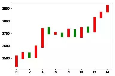
plt.figure()for i in range(0,15):
    dateOne = np.zeros([2])    # 建一个两列值为0的矩阵
    dateOne[0] = i;    # 第一列的 0-14
    dateOne[1] = i;    # 第二列的 0-14
    priceOne = np.zeros([2])    # 建一个两列值为0的矩阵
    priceOne[0] = beginPrice[i]    # 把开盘价输入第一列
    priceOne[1] = endPrice[i]    # 把收盘价输入第二列
    if endPrice[i] > beginPrice[i]:        # 如果收盘价 大于 开盘价
        plt.plot(dateOne,priceOne,'r',lw=8)        # 条形是红色，宽度为8
    else:
        plt.plot(dateOne,priceOne,'g',lw=8)        # 条形是绿色，宽度为8

结果：

函数解析：

1、range(start,stop,step)

• 只给一个参数 s,表示 从0到s
  例如：range(5)
  结果：[0,1,2,3,4]

• 两个参数,s,e,表示从s到e
  例如：range(5,10)
  结果：5,6,7,8,9

• 三个参数 s,e,i 表示从s到e，间隔i取数
  例如：range(0,10,2)
  结果：[0,2,4,6,8]

四、输入层 input layer

dateNormal = np.zeros([15,1])# 创建一个15行，1列的矩阵priceNormal = np.zeros([15,1])for i in range(0,15):
    dateNormal[i,0] = i/14.0;    # 日期的值，最大值为14
    priceNormal[i,0] = endPrice[i]/3000.0;    # 价格的值，最大值为3000x = tf.placeholder(tf.float32,[None,1])
y = tf.placeholder(tf.float32,[None,1])

函数解析：

tf.placeholder(dtype, shape=None, name=None)

• 解析：此函数可以理解为形参，用于定义过程，在执行的时候再赋具体的值

• 参数：
  dtype：数据类型。常用的是tf.float32,tf.float64等数值类型
  shape：数据形状。默认是None，就是一维值，也可以是**，比如[2,3], [None, 3]表示列是3，行不定
  name：名称。

• 返回：
  Tensor 类型

   

五、隐藏层（hidden layer）

w1 = tf.Variable(tf.random_uniform([1,10],0,1))
# 创建一个1行10列的矩阵，最小值为0，最大值为1
b1 = tf.Variable(tf.zeros([1,10]))
# 创建一个1行10列的矩阵，值都为0
wb1 = tf.matmul(x,w1)+b1
# wb1 = x * w1 + b1
layer1 = tf.nn.relu(wb1) 
# 激励函数的类型：
https://tensorflow.google.cn/api_guides/python/nn#Activation_Functions
# 激励函数的作用：
https://zhuanlan.zhihu.com/p/25279356

六、输出层（output layer）

w2 = tf.Variable(tf.random_uniform([10,1],0,1))
b2 = tf.Variable(tf.zeros([15,1]))
wb2 = tf.matmul(layer1,w2)+b2
# wb2 = wb1 * w2 + b2
layer2 = tf.nn.relu(wb2)

loss = tf.reduce_mean(tf.square(y-layer2))
# 计算真实值y和计算值layer2的标准差
# 方差 s^2=[(x1-x)^2+(x2-x)^2+......(xn-x)^2]/(n) （x为平均数）
# 标准差=方差的算术平方根
train_step = tf.train.GradientDescentOptimizer(0.1).minimize(loss)
# 每次梯度下降0.1，目的是缩小真实值y和计算值layer2的差值
with tf.Session() as sess:
    sess.run(tf.global_variables_initializer())
    for i in range(0,10000):
        sess.run(train_step,feed_dict={x:dateNormal,y:priceNormal})
        # feed_dict是一个字典，在字典中需要给出每一个用到的占位符的取值，每次迭代选取的数据只会拥有占位符这一个结点。
        # 训练出w1、w2、b1、b2，但是还需要检测是否有效
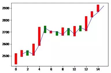
    pred = sess.run(layer2,feed_dict={x:dateNormal})
    # 训练完的预测结果值
    predPrice = np.zeros([15,1])
    for i in range(0,15):
        predPrice[i,0]=(pred*3000)[i,0]
        # pred需要乘以3000是因为前面 priceNormal[i,0] = endPrice[i]/3000.0;
    plt.plot(date,predPrice,'b',lw=1)
plt.show()

结果：

函数解析：

tf.reduce_mean(input_tensor,axis=None,keepdims=None,name=None,reduction_indices=None,keep_dims=None)

• 解析：计算张量维度上元素的平均值。

• 参数：
  input_tensor：张量减少。应该有数字类型。
  axis：要减小的尺寸。如果None（默认）缩小所有尺寸。必须在范围内 [ rank(input_tensor), rank(input_tensor) )。
  keepdims：如果为true，则保留长度为1的缩小尺寸。
  name：操作的名称（可选）。
  reduction_indices：轴的旧（已弃用）名称。
  keep_dims：已过时的别名keepdims。

延伸阅读：

使用Tensorflow预测股票市场变动