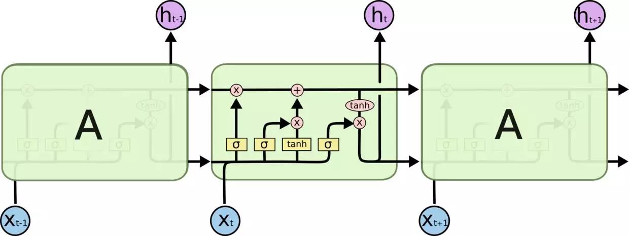
我们将解释如何建立一个有LSTM单元的RNN模型来预测S&P500指数的价格。 数据集可以从Yahoo!下载。 在例子中,使用了从1950年1月3日(Yahoo! Finance可以追溯到的最大日期)的S&P 500数据到2017年6月23日。 为了简单起见,我们只使用每日收盘价进行预测。 同时,我将演示如何使用TensorBoard轻松调试和模型跟踪。
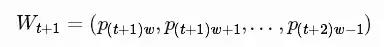
股票价格是长度为NN,定义为p0,p1,...,pN-1,其中pi是第i天的收盘价,0≤i<N。 我们有一个大小固定的移动窗口w(后面我们将其称为input_size),每次我们将窗口向右移动w个单位,以使所有移动窗口中的数据之间没有重叠。
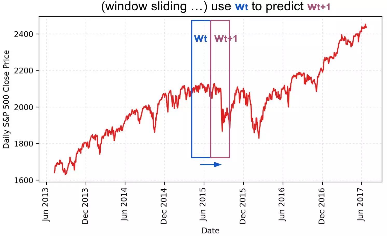
我们使用一个移动窗口中的内容来预测下一个,而在两个连续的窗口之间没有重叠。我们将建立RNN模型将LSTM单元作为基本的隐藏单元。 我们使用此值从时间t内将第一个移动窗口W0移动到窗口Wt:
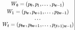
预测价格在下一个窗口在Wt+1
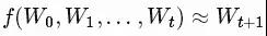
我们试图学习一个近似函数,
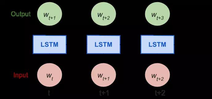
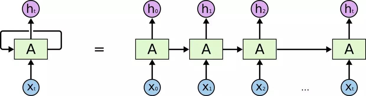
展开的RNN
考虑反向传播(BPTT)是如何工作的,我们通常将RNN训练成一个“unrolled”的样式,这样我们就不需要做太多的传播计算,而且可以节省训练的复杂性。以下是关于Tensorflow教程中input_size的解释:
By design, the output of a recurrent neural network (RNN) depends on arbitrarily distant inputs. Unfortunately, this makes backpropagation computation difficult. In order to make the learning process tractable, it is common practice to create an “unrolled” version of the network, which contains a fixed number (num_steps) of LSTM inputs and outputs. The model is then trained on this finite approximation of the RNN. This can be implemented by feeding inputs of length num_steps at a time and performing a backward pass after each such input block.
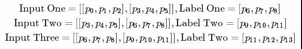
价格的顺序首先被分成不重叠的小窗口。 每个窗口都包含input_size数字,每个数字被视为一个**的输入元素。 然后,任何num_steps连续的输入元素被分配到一个训练输入中,形成一个训练在Tensorfow上的“unrolled”版本的RNN。 相应的标签就是它们后面的输入元素。例如,如果input_size = 3和num_steps = 2,我们的第一批的训练样例如下所示:
以下是数据格式化的关键部分:
seq = [np.array(seq[i * self.input_size: (i + 1) * self.input_size])
      for i in range(len(seq) // self.input_size)]

# Split into groups of `num_steps`
X = np.array([seq[i: i + self.num_steps] for i in range(len(seq) - self.num_steps)])
y = np.array([seq[i + self.num_steps] for i in range(len(seq) - self.num_steps)])
由于我们总是想预测未来,我们以最新的10%的数据作为测试数据。
标准普尔500指数随着时间的推移而增加,导致测试集中大部分数值超出训练集的范围,因此模型必须预测一些以前从未见过的数字。 但这却不是很理想。
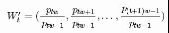
为了解决样本外的问题,我们在每个移动窗口中对价格进行了标准化。 任务变成预测相对变化率而不是绝对值。 在t时刻的标准化滑动窗口W't中,所有的值除以最后一个未知价格 Wt-1中的最后一个价格:
定义
lstm_size:一个LSTM图层中的单元数。
num_layers:堆叠的LSTM层的数量。
keep_prob:单元格在 dropout 操作中保留的百分比。
init_learning_rate:开始学习的速率。
learning_rate_decay:后期训练时期的衰减率。
init_epoch:使用常量init_learning_rate的时期数。
max_epoch:训练次数在训练中的总数
input_size:移动窗口的大小/一个训练数据点
batch_size:在一个小批量中使用的数据点的数量。
The LSTM model has num_layers stacked LSTM layer(s) and each layer contains lstm_sizenumber of LSTM cells. Then a dropout mask with keep probability keep_prob is applied to the output of every LSTM cell. The goal of dropout is to remove the potential strong dependency on one dimension so as to prevent overfitting.
The training requires max_epoch epochs in total; an epoch is a single full pass of all the training data points. In one epoch, the training data points are split into mini-batches of size batch_size. We send one mini-batch to the model for one BPTT learning. The learning rate is set to init_learning_rate during the first init_epoch epochs and then decay by learning_rate_decay during every succeeding epoch.
# Configuration is wrapped in one object for easy tracking and passing.
class RNNConfig():
   input_size=1
   num_steps=30
   lstm_size=128
   num_layers=1
   keep_prob=0.8
   batch_size = 64
   init_learning_rate = 0.001
   learning_rate_decay = 0.99
   init_epoch = 5
   max_epoch = 50

config = RNNConfig()
(1) Initialize a new graph first.
import tensorflow as tf
tf.reset_default_graph()
lstm_graph = tf.Graph()
(2) How the graph works should be defined within its scope.
with lstm_graph.as_default():
(3) Define the data required for computation. Here we need three input variables, all defined as tf.placeholder because we don’t know what they are at the graph construction stage.
inputs: the training data X, a tensor of shape (# data examples, num_steps, input_size); the number of data examples is unknown, so it is None. In our case, it would be batch_sizein training session. Check the input format example if confused.
targets: the training label y, a tensor of shape (# data examples, input_size).
learning_rate: a simple float.
# Dimension = (
   #     number of data examples,
   #     number of input in one computation step,
   #     number of numbers in one input
   # )
   # We don't know the number of examples beforehand, so it is None.
   inputs = tf.placeholder(tf.float32, [None, config.num_steps, config.input_size])
   targets = tf.placeholder(tf.float32, [None, config.input_size])
   learning_rate = tf.placeholder(tf.float32, None)
(4) This function returns one LSTMCell with or without dropout operation.
def _create_one_cell():
   return tf.contrib.rnn.LSTMCell(config.lstm_size, state_is_tuple=True)
   if config.keep_prob < 1.0:
           return tf.contrib.rnn.DropoutWrapper(lstm_cell, output_keep_prob=config.keep_prob)
(5) Let’s stack the cells into multiple layers if needed. MultiRNNCell helps connect sequentially multiple simple cells to compose one cell.
cell = tf.contrib.rnn.MultiRNNCell(
       [_create_one_cell() for _ in range(config.num_layers)],
       state_is_tuple=True
   ) if config.num_layers > 1 else _create_one_cell()
(6) tf.nn.dynamic_rnn constructs a recurrent neural network specified by cell (RNNCell). It returns a pair of (model outpus, state), where the outputs val is of size (batch_size, num_steps, lstm_size) by default. The state refers to the current state of the LSTM cell, not consumed here.
val, _ = tf.nn.dynamic_rnn(cell, inputs, dtype=tf.float32)
(7) tf.transpose converts the outputs from the dimension (batch_size, num_steps, lstm_size) to (num_steps, batch_size, lstm_size). Then the last output is picked.
# Before transpose, val.get_shape() = (batch_size, num_steps, lstm_size)
# After transpose, val.get_shape() = (num_steps, batch_size, lstm_size)
val = tf.transpose(val, [1, 0, 2])
# last.get_shape() = (batch_size, lstm_size)
ast = tf.gather(val, int(val.get_shape()[0]) - 1, name="last_lstm_output")
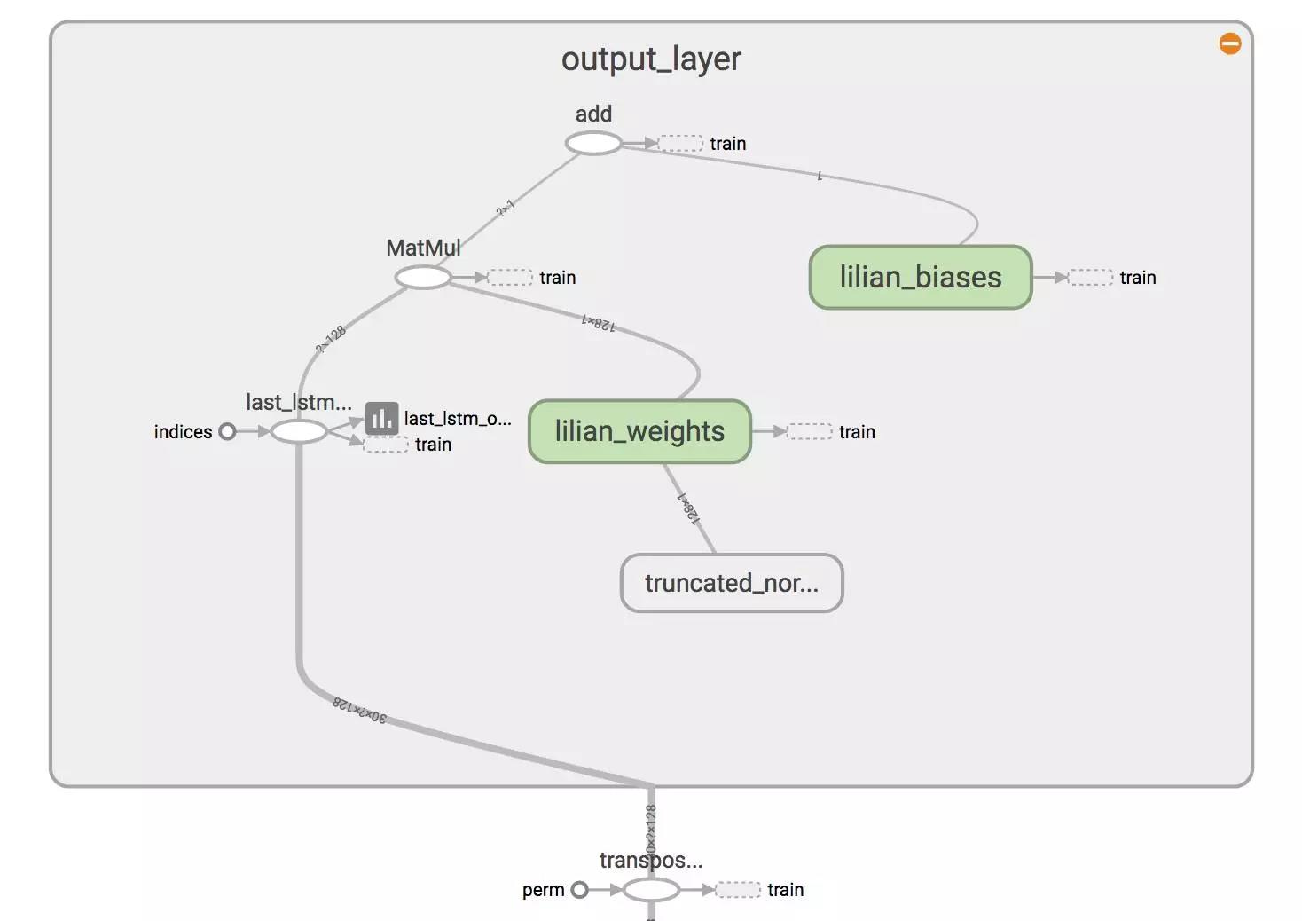
(8) Define weights and biases between the hidden and output layers.
weight = tf.Variable(tf.truncated_normal([config.lstm_size, config.input_size]))
bias = tf.Variable(tf.constant(0.1, shape=[targets_width]))
prediction = tf.matmul(last, weight) + bias
(9) We use mean square error as the loss metric and the RMSPropOptimizer algorithm for gradient descent optimization.(用手可以滑动代码)
loss = tf.reduce_mean(tf.square(prediction - targets))
optimizer = tf.train.RMSPropOptimizer(learning_rate)
minimize = optimizer.minimize(loss)
(1) To start training the graph with real data, we need to start a tf.session first.
with tf.Session(graph=lstm_graph) as sess:
(2) Initialize the variables as defined.
tf.global_variables_initializer().run()
(0) The learning rates for training epochs should have been precomputed beforehand. The index refers to the epoch index.(用手可以滑动代码
learning_rates_to_use = [
   config.init_learning_rate * (
       config.learning_rate_decay ** max(float(i + 1 - config.init_epoch), 0.0)
   ) for i in range(config.max_epoch)]
(3) Each loop below completes one epoch training.
for epoch_step in range(config.max_epoch):
   current_lr = learning_rates_to_use[epoch_step]

   # Check https://github.com/lilianweng/stock-rnn/blob/master/data_wrapper.py
   # if you are curious to know what is StockDataSet and how generate_one_epoch()
   # is implemented.
   for batch_X, batch_y in stock_dataset.generate_one_epoch(config.batch_size):
       train_data_feed = {
           nputs: batch_X,
           targets: batch_y,
           learning_rate: current_lr
       }
       train_loss, _ = sess.run([loss, minimize], train_data_feed)
(4) Don’t forget to save your trained model at the end.
saver = tf.train.Saver()
saver.save(sess, "your_awesome_model_path_and_name", global_step=max_epoch_step)
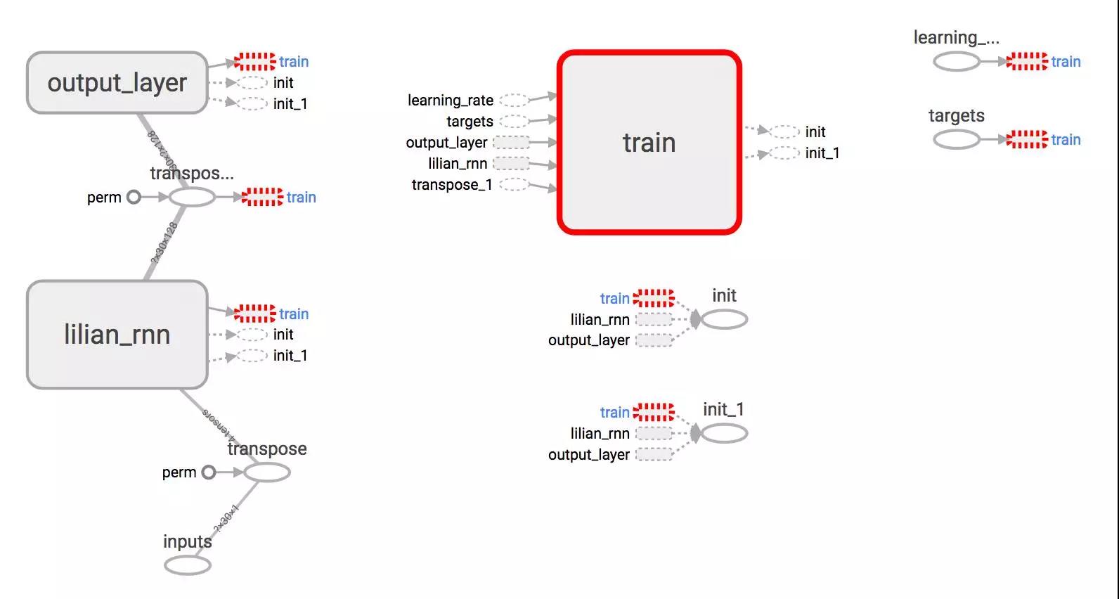
在没有可视化的情况下构建图形就像在黑暗中绘制,非常模糊和容易出错。 Tensorboard提供了图形结构和学习过程的简单可视化。 看看下面这个案例,非常实用:
Brief Summary
Use with [tf.name_scope](https://www.tensorflow.org/api_docs/python/tf/name_scope)("your_awesome_module_name"): to wrap elements working on the similar goal together.
Many tf.* methods accepts name= argument. Assigning a customized name can make your life much easier when reading the graph.
Methods like tf.summary.scalar and tf.summary.histogram help track the values of variables in the graph during iterations.
In the training session, define a log file using tf.summary.FileWriter.
with tf.Session(graph=lstm_graph) as sess:
   merged_summary = tf.summary.merge_all()
   writer = tf.summary.FileWriter("location_for_keeping_your_log_files", sess.graph)
   writer.add_graph(sess.graph)
Later, write the training progress and summary results into the file.
_summary = sess.run([merged_summary], test_data_feed)
writer.add_summary(_summary, global_step=epoch_step)  # epoch_step in range(config.max_epoch)
我们在例子中使用了以下配置。
num_layers=1
keep_prob=0.8
batch_size = 64
init_learning_rate = 0.001
learning_rate_decay = 0.99
init_epoch = 5
max_epoch = 100
num_steps=30
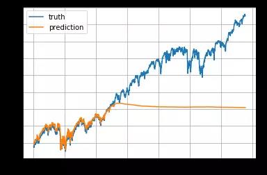
总的来说预测股价并不是一件容易的事情。 特别是在正则化后,价格趋势看起来非常嘈杂。
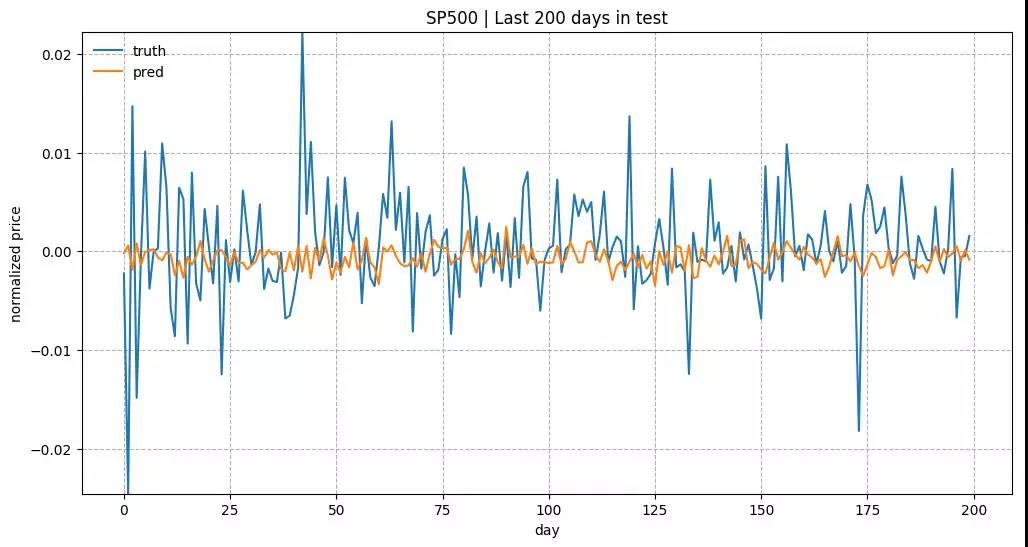
测试数据中最近200天的预测结果。 模型是用 input_size= 1 和 lstm_size= 32 来训练的。
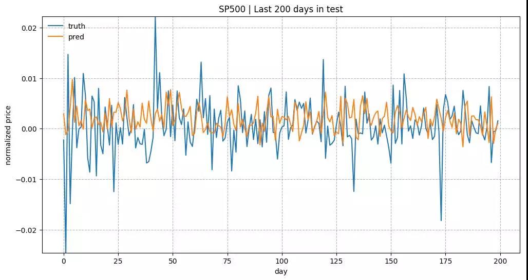
测试数据中最近200天的预测结果。 模型是用 input_size= 1 和 lstm_size= 128 来训练的。
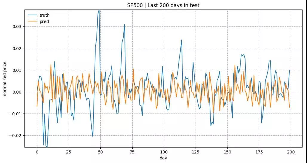
测试数据中最近200天的预测结果。 模型是用 input_size= 5 和 lstm_size= 128 来训练的。
代码:stock-rnn/main.py
import os
import pandas as pd
import pprint

import tensorflow as tf
import tensorflow.contrib.slim as slim

from data_model import StockDataSet
from model_rnn import LstmRNN

flags = tf.app.flags
flags.DEFINE_integer("stock_count", 100, "Stock count [100]")
flags.DEFINE_integer("input_size", 5, "Input size [5]")
flags.DEFINE_integer("num_steps", 30, "Num of steps [30]")
flags.DEFINE_integer("num_layers", 1, "Num of layer [1]")
flags.DEFINE_integer("lstm_size", 128, "Size of one LSTM cell [128]")
flags.DEFINE_integer("batch_size", 64, "The size of batch images [64]")
flags.DEFINE_float("keep_prob", 0.8, "Keep probability of dropout layer. [0.8]")
flags.DEFINE_float("init_learning_rate", 0.001, "Initial learning rate at early stage. [0.001]")
flags.DEFINE_float("learning_rate_decay", 0.99, "Decay rate of learning rate. [0.99]")
flags.DEFINE_integer("init_epoch", 5, "Num. of epoches considered as early stage. [5]")
flags.DEFINE_integer("max_epoch", 50, "Total training epoches. [50]")
flags.DEFINE_integer("embed_size", None, "If provided, use embedding vector of this size. [None]")
flags.DEFINE_string("stock_symbol", None, "Target stock symbol [None]")
flags.DEFINE_integer("sample_size", 4, "Number of stocks to plot during training. [4]")
flags.DEFINE_boolean("train", False, "True for training, False for testing [False]")

FLAGS = flags.FLAGS

pp = pprint.PrettyPrinter()

if not os.path.exists("logs"):
   os.mkdir("logs")


def show_all_variables():
   model_vars = tf.trainable_variables()
   slim.model_analyzer.analyze_vars(model_vars, print_info=True)


def load_sp500(input_size, num_steps, k=None, target_symbol=None, test_ratio=0.05):
   if target_symbol is not None:
       return [
           StockDataSet(
               target_symbol,
               input_size=input_size,
               num_steps=num_steps,
               test_ratio=test_ratio)
       ]

   # Load metadata of s & p 500 stocks
   info = pd.read_csv("data/constituents-financials.csv")
   info = info.rename(columns={col: col.lower().replace(' ', '_') for col in info.columns})
   info['file_exists'] = info['symbol'].map(lambda x: os.path.exists("data/{}.csv".format(x)))
   print info['file_exists'].value_counts().to_dict()

   info = info[info['file_exists'] == True].reset_index(drop=True)
   info = info.sort('market_cap', ascending=False).reset_index(drop=True)

   if k is not None:
       info = info.head(k)

   print "Head of S&P 500 info:\n", info.head()

   # Generate embedding meta file
   info[['symbol', 'sector']].to_csv(os.path.join("logs/metadata.tsv"), sep='\t', index=False)

   return [
       StockDataSet(row['symbol'],
                    input_size=input_size,
                    num_steps=num_steps,
                    test_ratio=0.05)
       for _, row in info.iterrows()]


def main(_):
   pp.pprint(flags.FLAGS.__flags)

   # gpu_options = tf.GPUOptions(per_process_gpu_memory_fraction=0.333)
   run_config = tf.ConfigProto()
   run_config.gpu_options.allow_growth = True

   with tf.Session(config=run_config) as sess:
       rnn_model = LstmRNN(
           sess,
           FLAGS.stock_count,
           lstm_size=FLAGS.lstm_size,
           num_layers=FLAGS.num_layers,
           num_steps=FLAGS.num_steps,
           input_size=FLAGS.input_size,
           keep_prob=FLAGS.keep_prob,
           embed_size=FLAGS.embed_size,
       )

       show_all_variables()

       stock_data_list = load_sp500(
           FLAGS.input_size,
           FLAGS.num_steps,
           k=FLAGS.stock_count,
           target_symbol=FLAGS.stock_symbol,
       )

       if FLAGS.train:
           rnn_model.train(stock_data_list, FLAGS)
       else:
           if not rnn_model.load()[0]:
               raise Exception("[!] Train a model first, then run test mode")


if __name__ == '__main__':
   tf.app.run()