在系列一的教程中,我们想继续有关股票价格预测的主题,并赋予在系列1中建立的具有对多个股票做出响应能力的RNN。 为了区分不同价格序列之间相关的模式,我们使用股票信号嵌入向量作为输入的一部分。
数据集
数据提取代码可以写成如下形式:
(用手可以滑动代码)
import urllib2
from datetime import datetime
BASE_URL = "https://www.google.com/finance/historical?"
          "output=csv&q={0}&startdate=Jan+1%2C+1980&enddate={1}"
symbol_url = BASE_URL.format(
   urllib2.quote('GOOG'), # Replace with any stock you are interested.
   urllib2.quote(datetime.now().strftime("%b+%d,+%Y"), '+')
)
在获取内容时,请记住在链接失败或提供的股票代码无效的情况下添加try-catch包装器。
(用手可以滑动代码)
try:
   f = urllib2.urlopen(symbol_url)
   with open("GOOG.csv", 'w') as fin:
       print >> fin, f.read()
except urllib2.HTTPError:
   print "Fetching Failed: {}".format(symbol_url)
建立模型
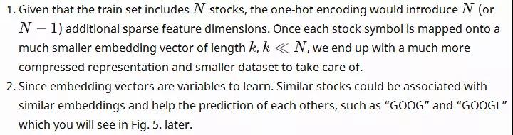
模型建立的预期是了解不同股票的价格序列。 由于不同的基本模式,我们想告诉模型应该操作哪一支股票。 嵌入(Embedding)比独热编码(one-hot encoding)更受欢迎,因为:
Embedding我们这里讲的通俗:从数学上的概念,从一个空间映射到另外一个空间,保留基本属性。比如把单词转化成向量,把数字(的奇偶正负实复等性质)转化成n维矩阵。
另一种选择是将嵌入向量与LSTM单元的最后状态连接,并在输出层中学习新的权重W和偏差b。 但是这样的话,LSTM单元就不能分辨出一只股票的价格,它的发挥就会受到很大的抑制。 于是我们决定采用前一种方法。
RNNConfig中添加了两个新的设置:
embedding_size控制每个嵌入向量的大小;
stock_symbol_size是指数据集中唯一股票的数量。
他们一起定义了嵌入矩阵的大小,模型必须学习embedding_size×stock_symbol_size附加变量与第一部分模型去比较。
(用手可以滑动代码)
class RNNConfig():
  # … old ones
  embedding_size = 8
  stock_symbol_size = 100
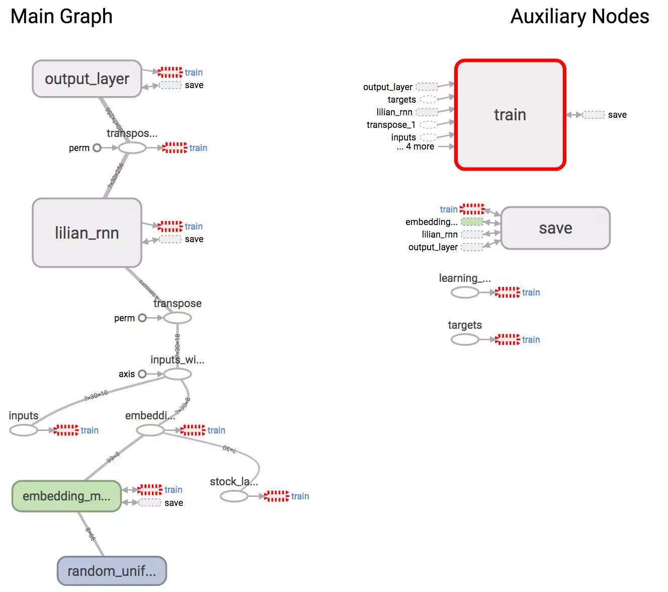
(1) As demonstrated in tutorial Part 1: Define the Graph, let us define a tf.Graph() named lstm_graph and a set of tensors to hold input data, inputs, targets, and learning_rate in the same way. One more placeholder to define is a list of stock symbols associated with the input prices. Stock symbols have been mapped to unique integers beforehand with label encoding.
(用手可以滑动代码)
# Mapped to an integer. one label refers to one stock symbol.
stock_labels = tf.placeholder(tf.int32, [None, 1])
(2)然后我们需要建立一个嵌入矩阵作为查找表,包含所有股票的嵌入向量。 矩阵在-1和1之间用随机数进行初始化,并在训练期间得到更新。
(用手可以滑动代码)
# Don’t forget: config = RNNConfig()
# Convert the integer labels to numeric embedding vectors.
embedding_matrix = tf.Variable(
       tf.random_uniform([config.stock_symbol_size, config.embedding_size], -1.0, 1.0)
   )
(3)重复股票标签 num_steps 次数来匹配训练期间unfolded的RNN和 inputs 张量的大小。 变换操作 tf.tile 接收一个基本张量,并创建一个新的张量,通过复制它的某个维度倍数;输入张量的第二维正好乘以 multiples[i] 倍。 例如,如果 stock_labels 为 [[0],[0],[2],[1]],则 [1,5] 产生 [[0 0 0 0 0],[0 0 0 0 0]) [2 2 2 2 2],[1 1 1 1 1 1]]。
(用手可以滑动代码)
stacked_stock_labels = tf.tile(stock_labels, multiples=[1, config.num_steps])
(4)然后根据查找表 embedding_matrix 将符号映射到嵌入向量。
(用手可以滑动代码)
# stock_label_embeds.get_shape() = (?, num_steps, embedding_size).
stock_label_embeds = tf.nn.embedding_lookup(embedding_matrix, stacked_stock_labels)
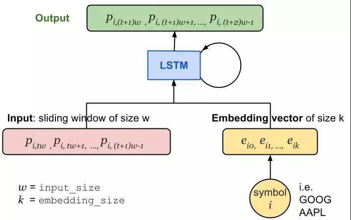
(5) Finally, combine the price values with the embedding vectors. The operation tf.concat concatenates a list of tensors along the dimension axis. In our case, we want to keep the batch size and the number of steps unchanged, but only extend the input vector of length input_size to include embedding features.
(用手可以滑动代码)
# inputs.get_shape() = (?, num_steps, input_size)
# stock_label_embeds.get_shape() = (?, num_steps, embedding_size)
# inputs_with_embed.get_shape() = (?, num_steps, input_size + embedding_size)
inputs_with_embed = tf.concat([inputs, stock_label_embeds], axis=2)
训练模型
第一部分部分请在下方查看:
系列一
在将数据送入图表之前,应该将股票符号转换为具有标签编码的唯一整数。
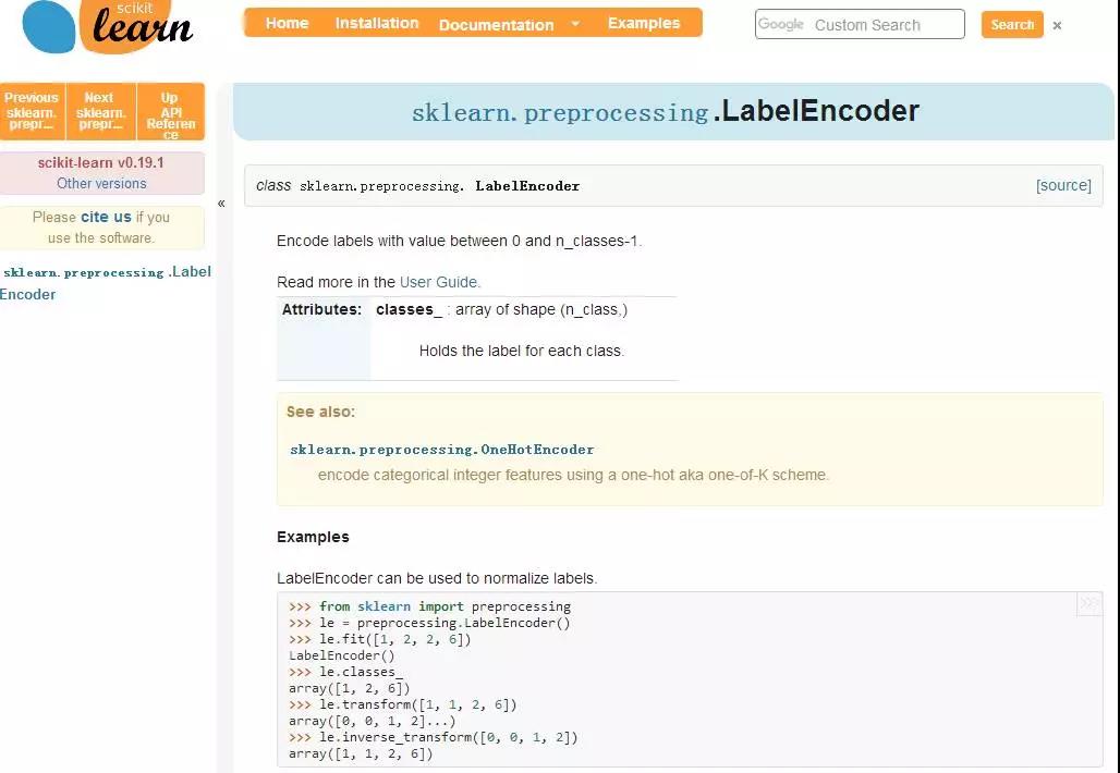
from sklearn.preprocessing import LabelEncoder
label_encoder = LabelEncoder()
label_encoder.fit(list_of_symbols)
训练/策略比例保持不变,90%用于训练,10%用于测试每个股票。
图形可视化
Other than presenting the graph structure or tracking the variables in time, Tensorboard also supports embeddings visualization. In order to communicate the embedding values to Tensorboard, we need to add proper tracking in the training logs.
(0) In my embedding visualization, I want to color each stock with its industry sector. This metadata should stored in a csv file. The file has two columns, the stock symbol and the industry sector. It does not matter whether the csv file has header, but the order of the listed stocks must be consistent with label_encoder.classes_.
(用手可以滑动代码)
import csv
embedding_metadata_path = os.path.join(your_log_file_folder, 'metadata.csv')
with open(embedding_metadata_path, 'w') as fout:
   csv_writer = csv.writer(fout)
   # write the content into the csv file.
   # for example, csv_writer.writerows(["GOOG", "information_technology"])
(1) Set up the summary writer first within the training tf.Session.
from tensorflow.contrib.tensorboard.plugins import projector
with tf.Session(graph=lstm_graph) as sess:
   summary_writer = tf.summary.FileWriter(your_log_file_folder)
   summary_writer.add_graph(sess.graph)
(2) Add the tensor embedding_matrix defined in our graph lstm_graph into the projector config variable and attach the metadata csv file.
(用手可以滑动代码)
projector_config = projector.ProjectorConfig()
# You can add multiple embeddings. Here we add only one.
added_embedding = projector_config.embeddings.add()
added_embedding.tensor_name = embedding_matrix.name
# Link this tensor to its metadata file.
added_embedding.metadata_path = embedding_metadata_path
(3) This line creates a file projector_config.pbtxt in the folder your_log_file_folder. TensorBoard will read this file during startup.
projector.visualize_embeddings(summary_writer, projector_config)
结果
该模型是在标准普尔500指数池里最大市值前100的股票进行训练。
input_size=10
num_steps=30
lstm_size=256
num_layers=1,
keep_prob=0.8
batch_size = 200
init_learning_rate = 0.05
learning_rate_decay = 0.99
init_epoch = 5
max_epoch = 500
embedding_size = 8
stock_symbol_size = 100
嵌入可视化
One common technique to visualize the clusters in embedding space is t-SNE (Maaten and Hinton, 2008),
which is well supported in Tensorboard. t-SNE, short for “t-Distributed Stochastic Neighbor Embedding, is a variation of Stochastic Neighbor Embedding (Hinton and Roweis, 2002),

but with a modified cost function that is easier to optimize.
Similar to SNE, t-SNE first converts the high-dimensional Euclidean distances between data points into conditional probabilities that represent similarities.
t-SNE defines a similar probability distribution over the data points in the low-dimensional space, and it minimizes the Kullback–Leibler divergence between the two distributions with respect to the locations of the points on the map.
Check (https://distill.pub/2016/misread-tsne/) for how to adjust the parameters, Perplexity and learning rate (epsilon), in t-SNE visualization.

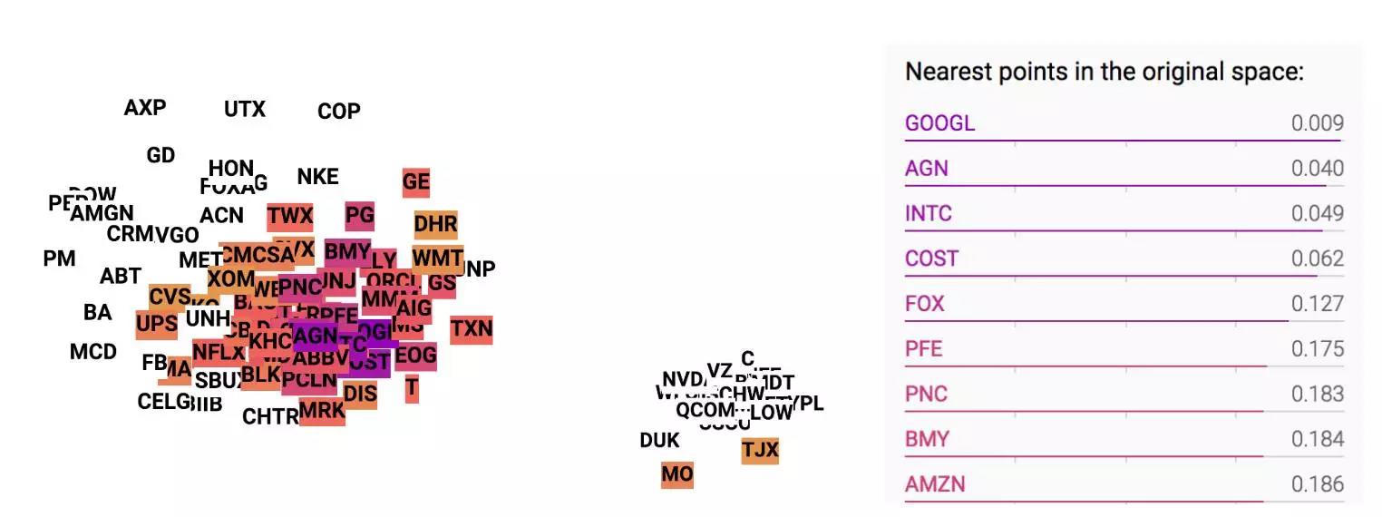
使用t-SNE可视化嵌入股票。 每个标签都是基于股票行业的颜色。
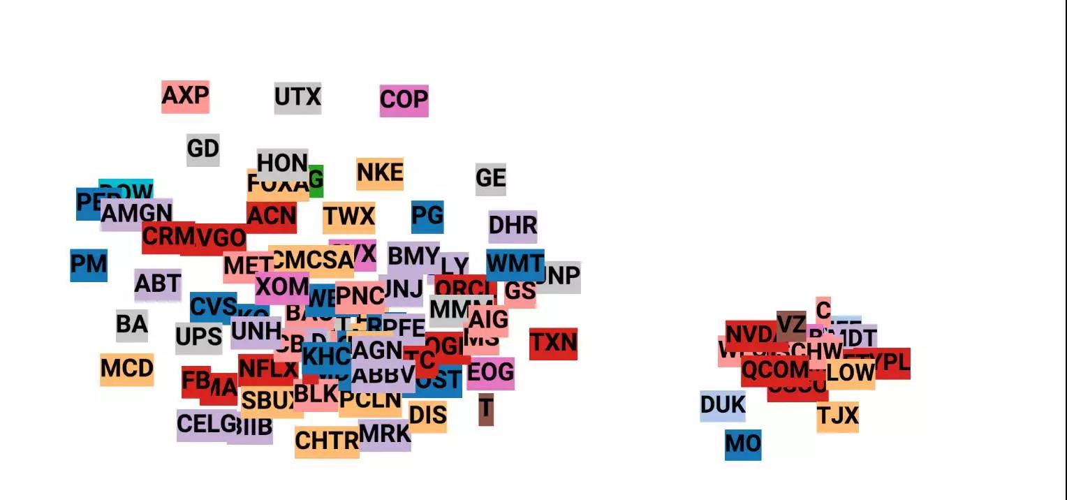
当我们在Tensorboard的嵌入标签中的“GOOG”时,其他相似的股票会随着相似度的下降在颜色上从暗到亮显现出来。
(用手可以滑动代码)
import numpy as np
import os
import random
import re
import shutil
import time
import tensorflow as tf
import matplotlib.pyplot as plt
from tensorflow.contrib.tensorboard.plugins import projector
class LstmRNN(object):
   def __init__(self, sess, stock_count,
                lstm_size=128,
                num_layers=1,
                num_steps=30,
                input_size=1,
                keep_prob=0.8,
                embed_size=None,
                logs_dir="logs",
                plots_dir="images"):
       """
       Construct a RNN model using LSTM cell.
       Args:
           sess:
           stock_count:
           lstm_size:
           num_layers
           num_steps:
           input_size:
           keep_prob:
           embed_size
           checkpoint_dir
       """
       self.sess = sess
       self.stock_count = stock_count

       self.lstm_size = lstm_size
       self.num_layers = num_layers
       self.num_steps = num_steps
       self.input_size = input_size
       self.keep_prob = keep_prob

       self.use_embed = (embed_size is not None) and (embed_size > 0)
       self.embed_size = embed_size or -1

       self.logs_dir = logs_dir
       self.plots_dir = plots_dir

       self.build_graph()

   def build_graph(self):
       """
       The model asks for three things to be trained:
       - input: training data X
       - targets: training label y
       - learning_rate:
       """
       # inputs.shape = (number of examples, number of input, dimension of each input).
       self.learning_rate = tf.placeholder(tf.float32, None, name="learning_rate")

       # Stock symbols are mapped to integers.
       self.symbols = tf.placeholder(tf.int32, [None, 1], name='stock_labels')

       self.inputs = tf.placeholder(tf.float32, [None, self.num_steps, self.input_size], name="inputs")
       self.targets = tf.placeholder(tf.float32, [None, self.input_size], name="targets")

       def _create_one_cell():
           lstm_cell = tf.contrib.rnn.LSTMCell(self.lstm_size, state_is_tuple=True)
           if self.keep_prob < 1.0:
               lstm_cell = tf.contrib.rnn.DropoutWrapper(lstm_cell, output_keep_prob=self.keep_prob)
           return lstm_cell

       cell = tf.contrib.rnn.MultiRNNCell(
           [_create_one_cell() for _ in range(self.num_layers)],
           state_is_tuple=True
       ) if self.num_layers > 1 else _create_one_cell()

       if self.embed_size > 0:
           self.embed_matrix = tf.Variable(
               tf.random_uniform([self.stock_count, self.embed_size], -1.0, 1.0),
               name="embed_matrix"
           )
           sym_embeds = tf.nn.embedding_lookup(self.embed_matrix, self.symbols)

           # stock_label_embeds.shape = (batch_size, embedding_size)
           stacked_symbols = tf.tile(self.symbols, [1, self.num_steps], name='stacked_stock_labels')
           stacked_embeds = tf.nn.embedding_lookup(self.embed_matrix, stacked_symbols)

           # After concat, inputs.shape = (batch_size, num_steps, lstm_size + embed_size)
           self.inputs_with_embed = tf.concat([self.inputs, stacked_embeds], axis=2, name="inputs_with_embed")
       else:
           self.inputs_with_embed = tf.identity(self.inputs)

       # Run dynamic RNN
       val, state_ = tf.nn.dynamic_rnn(cell, self.inputs, dtype=tf.float32, scope="dynamic_rnn")

       # Before transpose, val.get_shape() = (batch_size, num_steps, lstm_size)
       # After transpose, val.get_shape() = (num_steps, batch_size, lstm_size)
       val = tf.transpose(val, [1, 0, 2])

       last = tf.gather(val, int(val.get_shape()[0]) - 1, name="lstm_state")
       ws = tf.Variable(tf.truncated_normal([self.lstm_size, self.input_size]), name="w")
       bias = tf.Variable(tf.constant(0.1, shape=[self.input_size]), name="b")
       self.pred = tf.matmul(last, ws) + bias

       self.last_sum = tf.summary.histogram("lstm_state", last)
       self.w_sum = tf.summary.histogram("w", ws)
       self.b_sum = tf.summary.histogram("b", bias)
       self.pred_summ = tf.summary.histogram("pred", self.pred)

       # self.loss = -tf.reduce_sum(targets * tf.log(tf.clip_by_value(prediction, 1e-10, 1.0)))
       self.loss = tf.reduce_mean(tf.square(self.pred - self.targets), name="loss_mse")
       self.optim = tf.train.RMSPropOptimizer(self.learning_rate).minimize(self.loss, name="rmsprop_optim")

       self.loss_sum = tf.summary.scalar("loss_mse", self.loss)
       self.learning_rate_sum = tf.summary.scalar("learning_rate", self.learning_rate)

       self.t_vars = tf.trainable_variables()
       self.saver = tf.train.Saver()

   def train(self, dataset_list, config):
       """
       Args:
           dataset_list (<StockDataSet>)
           config (tf.app.flags.FLAGS)
       """
       assert len(dataset_list) > 0
       self.merged_sum = tf.summary.merge_all()

       # Set up the logs folder
       self.writer = tf.summary.FileWriter(os.path.join("./logs", self.model_name))
       self.writer.add_graph(self.sess.graph)

       if self.use_embed:
           # Set up embedding visualization
           # Format: tensorflow/tensorboard/plugins/projector/projector_config.proto
           projector_config = projector.ProjectorConfig()

           # You can add multiple embeddings. Here we add only one.
           added_embed = projector_config.embeddings.add()
           added_embed.tensor_name = self.embed_matrix.name
           # Link this tensor to its metadata file (e.g. labels).
           shutil.copyfile(os.path.join(self.logs_dir, "metadata.tsv"),
                           os.path.join(self.model_logs_dir, "metadata.tsv"))
           added_embed.metadata_path = "metadata.tsv"

           # The next line writes a projector_config.pbtxt in the LOG_DIR. TensorBoard will
           # read this file during startup.
           projector.visualize_embeddings(self.writer, projector_config)

       tf.global_variables_initializer().run()

       # Merged test data of different stocks.
       merged_test_X = []
       merged_test_y = []
       merged_test_labels = []

       for label_, d_ in enumerate(dataset_list):
           merged_test_X += list(d_.test_X)
           merged_test_y += list(d_.test_y)
           merged_test_labels += [[label_]] * len(d_.test_X)

       merged_test_X = np.array(merged_test_X)
       merged_test_y = np.array(merged_test_y)
       merged_test_labels = np.array(merged_test_labels)

       print "len(merged_test_X) =", len(merged_test_X)
       print "len(merged_test_y) =", len(merged_test_y)
       print "len(merged_test_labels) =", len(merged_test_labels)

       test_data_feed = {
           self.learning_rate: 0.0,
           self.inputs: merged_test_X,
           self.targets: merged_test_y,
           self.symbols: merged_test_labels,
       }

       global_step = 0

       num_batches = sum(len(d_.train_X) for d_ in dataset_list) // config.batch_size
       random.seed(time.time())

       # Select samples for plotting.
       sample_labels = range(min(config.sample_size, len(dataset_list)))
       sample_indices = {}
       for l in sample_labels:
           sym = dataset_list[l].stock_sym
           target_indices = np.array([
               i for i, sym_label in enumerate(merged_test_labels)
               if sym_label[0] == l])
           sample_indices[sym] = target_indices
       print sample_indices

       print "Start training for stocks:", [d.stock_sym for d in dataset_list]
       for epoch in xrange(config.max_epoch):
           epoch_step = 0
           learning_rate = config.init_learning_rate * (
               config.learning_rate_decay ** max(float(epoch + 1 - config.init_epoch), 0.0)
           )

           for label_, d_ in enumerate(dataset_list):
               for batch_X, batch_y in d_.generate_one_epoch(config.batch_size):
                   global_step += 1
                   epoch_step += 1
                   batch_labels = np.array([[label_]] * len(batch_X))
                   train_data_feed = {
                       self.learning_rate: learning_rate,
                       self.inputs: batch_X,
                       self.targets: batch_y,
                       self.symbols: batch_labels,
                   }
                   train_loss, _, train_merged_sum = self.sess.run(
                       [self.loss, self.optim, self.merged_sum], train_data_feed)
                   self.writer.add_summary(train_merged_sum, global_step=global_step)

                   if np.mod(global_step, len(dataset_list) * 100 / config.input_size) == 1:
                       test_loss, test_pred = self.sess.run([self.loss, self.pred], test_data_feed)

                       print "Step:%d [Epoch:%d] [Learning rate: %.6f] train_loss:%.6f test_loss:%.6f" % (
                           global_step, epoch, learning_rate, train_loss, test_loss)

                       # Plot samples
                       for sample_sym, indices in sample_indices.iteritems():
                           image_path = os.path.join(self.model_plots_dir, "{}_epoch{:02d}_step{:04d}.png".format(
                               sample_sym, epoch, epoch_step))
                           sample_preds = test_pred[indices]
                           sample_truth = merged_test_y[indices]
                           self.plot_samples(sample_preds, sample_truth, image_path, stock_sym=sample_sym)

                       self.save(global_step)

       final_pred, final_loss = self.sess.run([self.pred, self.loss], test_data_feed)

       # Save the final model
       self.save(global_step)
       return final_pred

   @property
   def model_name(self):
       name = "stock_rnn_lstm%d_step%d_input%d" % (
           self.lstm_size, self.num_steps, self.input_size)

       if self.embed_size > 0:
           name += "_embed%d" % self.embed_size

       return name

   @property
   def model_logs_dir(self):
       model_logs_dir = os.path.join(self.logs_dir, self.model_name)
       if not os.path.exists(model_logs_dir):
           os.makedirs(model_logs_dir)
       return model_logs_dir

   @property
   def model_plots_dir(self):
       model_plots_dir = os.path.join(self.plots_dir, self.model_name)
       if not os.path.exists(model_plots_dir):
           os.makedirs(model_plots_dir)
       return model_plots_dir

   def save(self, step):
       model_name = self.model_name + ".model"
       self.saver.save(
           self.sess,
           os.path.join(self.model_logs_dir, model_name),
           global_step=step
       )

   def load(self):
       print(" [*] Reading checkpoints...")
       ckpt = tf.train.get_checkpoint_state(self.model_logs_dir)
       if ckpt and ckpt.model_checkpoint_path:
           ckpt_name = os.path.basename(ckpt.model_checkpoint_path)
           self.saver.restore(self.sess, os.path.join(self.model_logs_dir, ckpt_name))
           counter = int(next(re.finditer("(\d+)(?!.*\d)", ckpt_name)).group(0))
           print(" [*] Success to read {}".format(ckpt_name))
           return True, counter

       else:
           print(" [*] Failed to find a checkpoint")
           return False, 0

   def plot_samples(self, preds, targets, figname, stock_sym=None):
       def _flatten(seq):
           return [x for y in seq for x in y]

       truths = _flatten(targets)[-200:]
       preds = _flatten(preds)[-200:]
       days = range(len(truths))[-200:]

       plt.figure(figsize=(12, 6))
       plt.plot(days, truths, label='truth')
       plt.plot(days, preds, label='pred')
       plt.legend(loc='upper left', frameon=False)
       plt.xlabel("day")
       plt.ylabel("normalized price")
       plt.ylim((min(truths), max(truths)))
       plt.grid(ls='--')

       if stock_sym:
           plt.title(stock_sym + " | Last %d days in test" % len(truths))

       plt.savefig(figname, format='png', bbox_inches='tight', transparent=True)
       plt.close()