套利定价理论是一个重要的资产定价理论,它是用线性因子模型来表达收益率的:Ri=ai+bi1F1+bi2F2+…+biKFK+ϵiRi=ai+bi1F1+bi2F2+…+biKFK+ϵi
这一理论指出,如果收益率符合如上模型,那么期望收益率则符合如下模型E(Ri)=RF+bi1λ1+bi2λ2+…+biKλKE(Ri)=RF+bi1λ1+bi2λ2+…+biKλK
RFRF是无风险利率,λjλj是风险溢价,即收益率中超过无风险利率部分,jj代表第j个因子。溢价的存在是因为投资者要求更高的回报来补偿他们所多承担的风险。这就推广了资本资产定价模型(CAPM),CAPM仅使用市场上收益率作为其惟一的影响因子。
为了计算λjλj,我们可以构造一个灵敏度对因子j为1但对其他因子为0的投资组合(即j因子的纯因子组合),然后计算它的风险溢价。或者,我们对K个充分分散的(没有资产特定风险 即ϵp=0ϵp=0)资产组合计算灵敏度,然后解线性方程组求得λjλj。
套利
我们的世界里有许许多多的证券。如果我们使用不同的证券计算λλ,我们的结果会一致吗?如果不一致的话,那就存在套利的机会(在期望上)。套利是一种没有风险、净投资为0、期望收益为正的操作行为,而一个套利机会就是一个能进行套利的机会。套利发生时机是预期收益不一致时,即证券市场对风险定价不一致时。
例如,一个套利机会存在于以下情况下:一个资产明年的期望收益率是0.2 ,相对市场因子的ββ是1.2,而市场期望收益率为0.1,1年期债券的无风险利率是0.05。那么,利用APT模型可以得到资产的期望收益率为RF+βλ=0.05+1.2(0.1−0.05)=0.11RF+βλ=0.05+1.2(0.1−0.05)=0.11
这和资产的期望收益率0.2并不一致。所以,如果我们购买100美元的资产,从市场借入120美元,买入20美元的债券,无需资金上的净投入,我们没有承担任何的系统性风险(我们是市场中性的),但年底,我们在期望下能赚 0.2⋅100−0.1⋅120+20⋅0.05=90.2⋅100−0.1⋅120+20⋅0.05=9 。套利定价理论假设认为,套利机会将会被一直利用,直到价格改变,机会消失。也就是说,它假设在市场中总存在一群有足够的耐心和资本的套利者在套利。这为使用实证因子模型进行证券定价提供了一种辩护词:如果模型矛盾,是因为还有套利机会,价格还将会改变。
两头操作
通常,想知道E(Ri)E(Ri)是非常困难的,但请注意,这个模型能够告诉我们答案,如果市场被充分套利的话。这为基于因子模型排名系统的长短仓策略奠定了基础。如果你知道一个资产在市场被套利下的期望收益率,并且假设在你交易的时间都处于市场被套利下,然后你就可以建立一个排名。
长短仓
要做到这个,要估计市场上每个资产的期望回报率,然后排名。买入前几名,卖出后几名,你靠其中收益率的差异赚到钱。换言之,如果排名最靠前的资产能每年比市场平均水平多5%5%的收益率,而最靠后的资产会少5%5%,那么你将每年收益(M+0.05)−(M−0.05)=0.10(M+0.05)−(M−0.05)=0.10 即 10%10%,其中市场收益率MM被抵消了。长短仓的思想是,虽然单个资产很难模拟,但大的趋势却可以。我们不能准确地预测资产的期望收益,但我们能预测一组包括1000个资产的组合的期望收益率,因为误差被分摊了。我们以后将会用一整个章节来讲长短仓。
你想要多少的因子?
正如其他章节所探讨的,过度拟合,即更多的因子将更能解释你的收益率,但代价是数据中的噪音也被拟合了。为了发现真正的信号和准确地预测未来,你会想选择尽可能少的参数,但仍然能解释收益率的方差中的大部分。
例子:计算两种资产的期望收益率
In [3]:
import numpy as np
import pandas as pd
from statsmodels import regression
import matplotlib.pyplot as plt
让我们导入一些数据。
In [4]:
start_date = '2014-06-30'
end_date = '2015-06-30'

# 我们向未来多看一个月的数据
offset_start_date = '2014-07-31'
offset_end_date = '2015-07-31'

# 获得资产的收益率
# asset1 = get_pricing('HSC', fields='price', start_date=offset_start_date, end_date=offset_end_date).pct_change()[1:]
# asset2 = get_pricing('MSFT', fields='price', start_date=offset_start_date, end_date=offset_end_date).pct_change()[1:]
asset1 = get_price('000001.XSHE', start_date=offset_start_date, end_date=offset_end_date,frequency='daily',fields='price')['price'].pct_change()[1:]
asset2 = get_price('000002.XSHE', start_date=offset_start_date, end_date=offset_end_date,frequency='daily',fields='price')['price'].pct_change()[1:]

# 获得市场的收益率
#bench = get_pricing('SPY', fields='price', start_date=start_date, end_date=end_date).pct_change()[1:]
bench = get_price('510300.XSHG', start_date=start_date, end_date=end_date,frequency='daily',fields='price')['price'].pct_change()[1:]

# 用上证5年期国债ETF的十分之一作为无风险利率(缺数据,以此暂时替代)
# treasury_ret = get_pricing('BIL', fields='price', start_date=start_date, end_date=end_date).pct_change()[1:]
treasury_ret = get_price('511010.XSHG', start_date=start_date, end_date=end_date,frequency='daily',fields='price')['price'].pct_change()[1:]/10
In [5]:
# 定义一个常量来计算截距
constant = pd.TimeSeries(np.ones(len(asset1.index)), index=asset1.index)

df = pd.DataFrame({'R1': asset1,
              'R2': asset2,
              'SPY': bench,
              'RF': treasury_ret,
              'Constant': constant})
df = df.dropna()
我们首先进行整个时期的静态回归。
In [6]:
OLS_model = regression.linear_model.OLS(df['R1'], df[['SPY', 'RF', 'Constant']])
fitted_model = OLS_model.fit()
print 'p-value', fitted_model.f_pvalue
print fitted_model.params
R1_params = fitted_model.params

OLS_model = regression.linear_model.OLS(df['R2'], df[['SPY', 'RF', 'Constant']])
fitted_model = OLS_model.fit()
print 'p-value', fitted_model.f_pvalue
print fitted_model.params
R2_params = fitted_model.params
p-value 8.74334096699e-39
SPY 1.039088
RF -9.529748
Constant -0.000300
dtype: float64
p-value 2.13373128261e-36
SPY 1.113869
RF -3.833639
Constant -0.000995
dtype: float64
就像我们之前在其他章节说的,这些数字本身并没有告诉我们很多。我们需要看估计系数的分布,以及它是否稳定。让我们做90天的滚动回归看看怎么样。
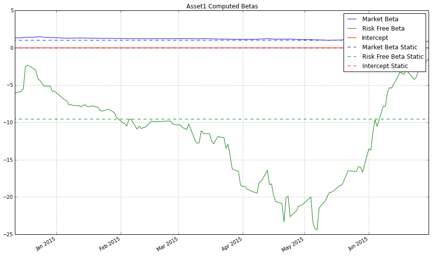
In [8]:
model = pd.stats.ols.MovingOLS(y = df['R1'], x=df[['SPY', 'RF']],
                             window_type='rolling',
                             window=90)

rolling_parameter_estimates = model.beta
rolling_parameter_estimates.plot(figsize=[15,9],grid='on')

plt.hlines(R1_params['SPY'], df.index[0], df.index[-1], linestyles='dashed', colors='blue')
plt.hlines(R1_params['RF'], df.index[0], df.index[-1], linestyles='dashed', colors='green')
plt.hlines(R1_params['Constant'], df.index[0], df.index[-1], linestyles='dashed', colors='red')


plt.title('Asset1 Computed Betas');
plt.legend(['Market Beta', 'Risk Free Beta', 'Intercept', 'Market Beta Static', 'Risk Free Beta Static', 'Intercept Static']);
In [9]:
model = pd.stats.ols.MovingOLS(y = df['R2'], x=df[['SPY', 'RF']],
                             window_type='rolling',
                             window=90)
rolling_parameter_estimates = model.beta
rolling_parameter_estimates.plot(figsize=[15,9],grid='on');

plt.hlines(R2_params['SPY'], df.index[0], df.index[-1], linestyles='dashed', colors='blue')
plt.hlines(R2_params['RF'], df.index[0], df.index[-1], linestyles='dashed', colors='green')
plt.hlines(R2_params['Constant'], df.index[0], df.index[-1], linestyles='dashed', colors='red')

plt.title('Asset2 Computed Betas');
plt.legend(['Market Beta', 'Risk Free Beta', 'Intercept', 'Market Beta Static', 'Risk Free Beta Static', 'Intercept Static']);
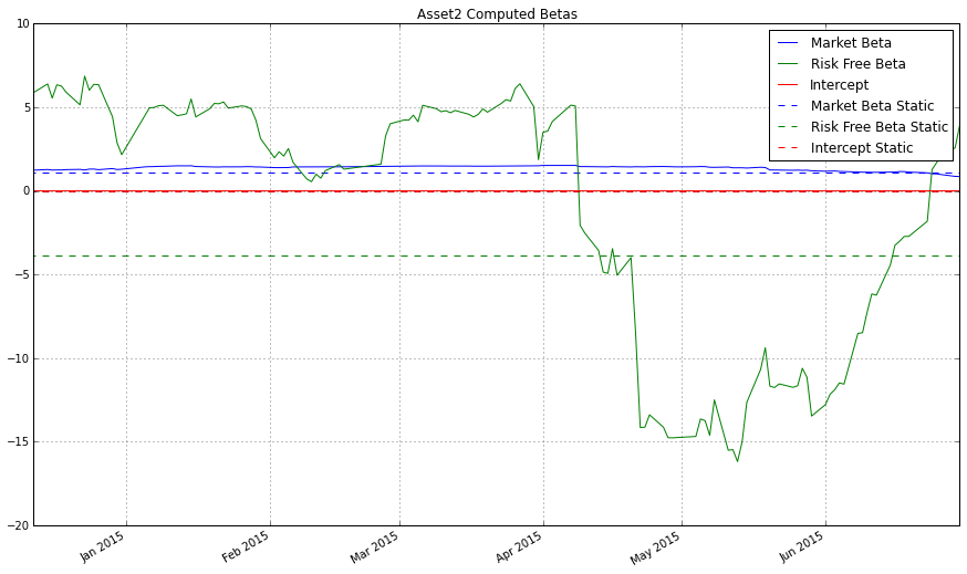
市场贝塔看起来是挺稳定的,但是让我们放大来检查检查。
In [10]:
model = pd.stats.ols.MovingOLS(y = df['R2'], x=df[['SPY', 'RF']],
                             window_type='rolling',
                             window=90)
rolling_parameter_estimates = model.beta
rolling_parameter_estimates['SPY'].plot(figsize=[15,9],grid='on');

plt.hlines(R2_params['SPY'], df.index[0], df.index[-1], linestyles='dashed', colors='blue')

plt.title('Asset2 Computed Betas');
plt.legend(['Market Beta', 'Market Beta Static']);
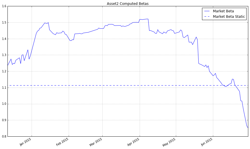
正如你所看到的,绘图的比例大大地影响我们对估计质量的认知。
让我们用这个模型来预测这些资产的价格。
In [11]:
start_date = '2014-07-25'
end_date = '2015-07-25'

# 我们向未来看一个月的数据
offset_start_date = '2014-08-25'
offset_end_date = '2015-08-25'

# 取得资产收益率数据
# asset1 = get_pricing('HSC', fields='price', start_date=offset_start_date, end_date=offset_end_date).pct_change()[1:]
asset1 = get_price('000001.XSHE', start_date=offset_start_date, end_date=offset_end_date,frequency='daily',fields='price')['price'].pct_change()[1:]

# 取得市场收益率
#bench = get_pricing('SPY', fields='price', start_date=start_date, end_date=end_date).pct_change()[1:]
bench = get_price('510300.XSHG', start_date=start_date, end_date=end_date,frequency='daily',fields='price')['price'].pct_change()[1:]

# 用上证5年期国债ETF的十分之一作为无风险利率(缺数据,以此暂时替代)
# treasury_ret = get_pricing('BIL', fields='price', start_date=start_date, end_date=end_date).pct_change()[1:]
treasury_ret = get_price('511010.XSHG', start_date=start_date, end_date=end_date,frequency='daily',fields='price')['price'].pct_change()[1:]/10

# 定义一个常量计算截距
constant = pd.TimeSeries(np.ones(len(asset1.index)), index=asset1.index)

df = pd.DataFrame({'R1': asset1,
              'SPY': bench,
              'RF': treasury_ret,
              'Constant': constant})
df = df.dropna()
我们将做一个历史回归得到模型参数的估计值。
In [12]:
OLS_model = regression.linear_model.OLS(df['R1'], df[['SPY', 'RF', 'Constant']])
fitted_model = OLS_model.fit()
print 'p-value', fitted_model.f_pvalue
print fitted_model.params

b_SPY = fitted_model.params['SPY']
b_RF = fitted_model.params['RF']
a = fitted_model.params['Constant']
p-value 6.97733078778e-35
SPY         0.841368
RF         -4.186051
Constant    0.000133
dtype: float64
获得上个月因子的数据,然后,我们来预测下个月。
In [13]:
start_date = '2015-07-25'
end_date = '2015-08-25'

# 取得市场收益率
# last_month_bench = get_pricing('SPY', fields='price', start_date=start_date, end_date=end_date).pct_change()[1:]
last_month_bench = get_price('510300.XSHG', start_date=start_date, end_date=end_date,frequency='daily',fields='price')['price'].pct_change()[1:]

# 用上证5年期国债ETF的十分之一作为无风险利率(缺数据,以此暂时替代)
# last_month_treasury_ret = get_pricing('BIL', fields='price', start_date=start_date, end_date=end_date).pct_change()[1:]
last_month_treasury_ret = get_price('511010.XSHG', start_date=start_date, end_date=end_date,frequency='daily',fields='price')['price'].pct_change()[1:]/10
做出我们的预测。
In [14]:
predictions = b_SPY * last_month_bench + b_RF * last_month_treasury_ret + a
predictions.index = predictions.index + pd.DateOffset(months=1)
In [15]:
plt.figure(figsize=[15,9])
plt.grid(True)
plt.plot(asset1.index[-30:], asset1.values[-30:], 'b-')
plt.plot(predictions.index, predictions, 'b--')
plt.ylabel('Returns')
plt.legend(['Actual', 'Predicted']);
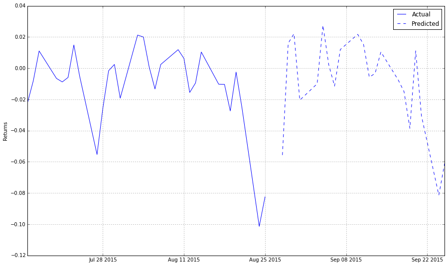
当然,这个分析还没有告诉我们这次预测质量怎么样。检查它我们需要使用,如样本外测试或交叉验证等技术。至于检验长短仓排名系统,斯皮尔曼等级相关的章节详细讲解了如何检验一个排名系统。
重要提醒!
再说一次,任何单独一次的预测很可能是不准的。实业品质的建模是对千上万的资产进行预测,并广泛的持仓。如果我告诉你一个预测成功率为51%模型,你不应该为一次预测,赌上你所有的钱。你应该做出成千上万次的预测,然后把你的钱在其中分散开来。
 1人赞赏收藏