R语言常用上机命令分功能整理——时间序列分析为主

第一讲

应用实例

• R的基本界面是一个交互式命令窗口，命令提示符是一个大于号，命令的结果马上显示在命令下面。

• S命令主要有两种形式：表达式或赋值运算（用’<－’或者’=’表示）。在命令提示符后键入一个表达式表示计算此表达式并显示结果。赋值运算把赋值号右边的值计算出来赋给左边的变量。
• 可以用向上光标键来找回以前运行的命令再次运行或修改后再运行。
• S是区分大小写的，所以x和X是不同的名字。

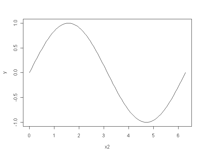
我们用一些例子来看R软件的特点。假设我们已经进入了R的交互式窗口。如果没有打开的图形窗口，在R中，用：> x11() 可以打开一个作图窗口。然后，输入以下语句：

x1 = 0:100

x2 = x1*2*pi/100

y = sin(x2)

plot(x2,y,type="l")

 

这些语句可以绘制正弦曲线图。其中，“=”是赋值运算符。0:100表示一个从0到100 的等差数列向量。第二个语句可以看出，我们可以对向量直接进行四则运算，计算得到的x2 是向量x1的所有元素乘以常数2*pi/100的结果。从第三个语句可看到函数可以以向量为输入，并可以输出一个向量，结果向量y的每一个分量是自变量x2的每一个分量的正弦函数值。

plot(x2,y, type="l",main="画图练习",sub="好好练", xlab="x轴",ylab='y轴')

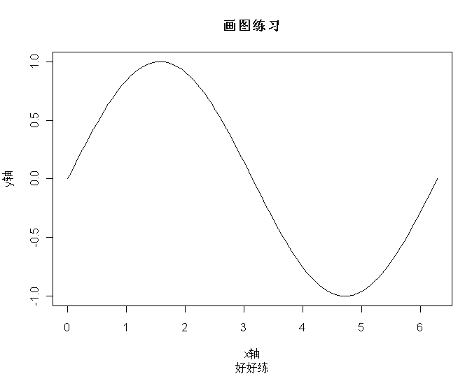
有关作图命令plot的详细介绍可以在R中输入help(plot)

 

 

 

数学函数

abs，sqrt：绝对值，平方根 log, log10, log2 , exp：对数与指数函数 sin，cos，tan，asin，acos，atan，atan2：三角函数 sinh，cosh，tanh，asinh，acosh，atanh：双曲函数

 

简单统计量

sum, mean, var, sd, min, max, range, median, IQR（四分位间距）等为统计量，sort，order，rank与排序有关，其它还有ave，fivenum，mad，quantile，stem等。

 

下面我们看一看S的统计功能:

> marks <- c(10, 6, 4, 7, 8)

> mean(marks)

> sd(marks)

> min(marks)

> max(marks)

 

第一个语句输入若干数据到一个向量，函c()用来把数据组合为一个向量。后面用了几个函数来计算数据的均值、标准差、最小值、最大值。

 

可以把若干行命令保存在一个文本文件中，然后用source函数来运行整个文件：

> source("C:/l.R")

          注意字符串中的反斜杠。

 

例:计算6, 4, 7, 8，10的均值和标准差，把若干行命令保存在一个文本文件（比如C:\1.R）中，然后用source函数来运行整个文件。

a<- c(10, 6, 4, 7, 8)

b<-mean(a)

c<-sd(a)

source("C:/1.R")

 

时间序列数据的输入

使用函数ts

ts(1:10, frequency = 4, start = c(1959, 2))

print( ts(1:10, frequency = 7, start = c(12, 2)), calendar = TRUE)

a<-ts(1:10, frequency = 4, start = c(1959, 2))

plot(a)

 

 

将外部数据读入R

read.csv

默认header = TRUE，也就是第一行是标签，不是数据。

read.table

默认header = FALSE

 

将R中的数据输出

write

write.table
write.csv

 

第二讲

1. 绘制时序图、自相关图

例题2.1

d=scan("sha.csv")

sha=ts(d,start=1964,freq=1)

plot.ts(sha)   #绘制时序图

acf(sha,22)   #绘制自相关图，滞后期数22

pacf(sha,22)  #绘制偏自相关图，滞后期数22

corr=acf(sha,22)   #保存相关系数

cov=acf(sha,22,type = "covariance")   #保存协方差

图的保存，单击选中图，在菜单栏选中“文件”，再选“另存为”。

同时显示多个图：用x11()命令生成一个空白图，再输入作图命令。

 

2. 同时绘制两组数据的时序图

d=read.csv("double.csv",header=F)

double=ts(d,start=1964,freq=1)

plot(double, plot.type = "multiple")   #两组数据两个图

plot(double, plot.type = "single")     #两组数据一个图

plot(double, plot.type = "single",col=c("red","green"),lty=c(1,2)) #设置每组数据图的颜色、曲线类型)

 

3.产生服从正态分布的随机观察值

例题2.4 随机产生1000白噪声序列观察值

d=rnorm(1000,0,1)   #个数1000 均值0 方差1

plot.ts(d)

 

4.纯随机性检验

例题2.3续

d=scan("temp.csv")

temp=ts(d,freq=1,start=c(1949))

Box.test(temp, type="Ljung-Box",lag=6)

 

5.差分计算

x=1:10

y=diff(x)

k步差分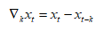 加入参数 lag=k

如计算x的3步差分为

y=diff(x, lag = 3)

p阶差分 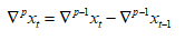加入参数differences = p

如2阶差分

y=diff(x,differences = 2)

 

第三讲

例题3.1

plot.ts(arima.sim(n = 100, list(ar = 0.8)))

#模拟AR(1)模型，并作时序图。

plot.ts(arima.sim(n = 100, list(ar = -1.1)))

#非平稳，无法得到时序图。

plot.ts(arima.sim(n = 100, list(ar = c(1,-0.5))))

plot.ts(arima.sim(n = 100, list(ar = c(1,0.5))))

 

例题3.5

acf(arima.sim(n = 100, list(ar = 0.8)))

acf (arima.sim(n = 100, list(ar = -1.1)))

acf (arima.sim(n = 100, list(ar = c(1,-0.5))))

acf (arima.sim(n = 100, list(ar = c(1,0.5))))

 

例题3.7

arima.sim(n = 1000, list(ar = 0.5, ma = -0.8))

acf(arima.sim(n = 1000, list(ar = 0.5, ma = -0.8)),20)

pacf(arima.sim(n = 1000, list(ar = 0.5, ma = -0.8)),20)

 

例题2.5

d=scan("a1.5.txt")               #导入数据

prop=ts(d,start=1950,freq=1)      #转化为时间序列数据

plot(prop)                   #作时序图

acf(prop,12)                 #作自相关图，拖尾

pacf(prop,12)                #作偏自相关图，1阶截尾

Box.test(prop, type="Ljung-Box",lag=6) 

#纯随机性检验,p值小于5%，序列为非白噪声

Box.test(prop, type="Ljung-Box",lag=12)

arima(prop, order = c(1,0,0),method="ML")

#用AR(1)模型拟合，如参数method="CSS"，估计方法为条件最小二乘法，用条件最小二乘法时，不显示AIC。

arima(prop, order = c(1,0,0),method="ML", include.mean = F) #用AR(1)模型拟合，不含截距项。

tsdiag(arima(prop, order = c(1,0,0),method="ML")) 

#对估计进行诊断，判断残差是否为白噪声

summary(arima(prop, order = c(1,0,0),method="ML"))

a=arima(prop, order = c(1,0,0),method="ML")

r=a$residuals#用r来保存残差

Box.test(r,type="Ljung-Box",lag=6)#对残差进行纯随机性检验

predict(arima(prop, order = c(1,0,0)), n.ahead =5)   #预测未来5期

prop.fore = predict(arima(prop, order = c(1,0,0)), n.ahead =5)

#将未来5期预测值保存在prop.fore变量中

U = prop.fore$pred + 1.96* prop.fore$se

L = prop.fore$pred – 1.96* prop.fore$se#算出95%置信区间

ts.plot(prop, prop.fore$pred,col=1:2)#作时序图，含预测。

lines(U, col="blue", lty="dashed")

lines(L, col="blue", lty="dashed")#在时序图中作出95%置信区间

 

例题3.9

d=scan("a1.22.txt")

x=diff(d)

arima(x, order = c(1,0,1),method="CSS")

tsdiag(arima(x, order = c(1,0,1),method="CSS"))

 

第一点：

对于第三讲中的例2.5，运行命令arima(prop, order = c(1,0,0),method="ML")之后，显示：

Call:

arima(x = prop, order = c(1, 0, 0), method = "ML")

Coefficients:

         ar1    intercept

      0.6914    81.5509

s.e.   0.0989     1.7453

sigma^2 estimated as 15.51:  log likelihood = -137.02,  aic = 280.05

 

注意：intercept下面的81.5509是均值，而不是截距！虽然intercept是截距的意思，这里如果用mean会更好。（the mean and the intercept are the same only when there is no AR term，均值和截距是相同的，只有在没有AR项的时候）

如果想得到截距，利用公式计算。int=(1-0.6914)*81.5509= 25.16661。课本P81的例2.5续中的截距25.17是正确的。

 

 

第二点：

如需计算参数的t统计量值和p值，利用下面的公式。

ar的t统计量值=0.6914/0.0989= 6.9909

(注：数值与课本略有不同，因为课本用sas算的se= 0.1029，R计算的se=0.0989)

p值=pt(6.9909,df=48,lower.tail = F)*2

pt()为求t分布求p值的函数，6.99为t统计量的绝对值，df为自由度=数据个数-参数个数，lower.tail = F表示所求p值为P[T > t]，如不加入这个参数表示所求p值为P[T <=t]。

乘2表示p值是双侧的（课本上的p值由sas算出，是双侧的）

 

均值的t统计量值和p值同理。

 

在时间序列中对参数显著性的要求与回归模型不同，我们更多的是考察模型整体的好坏，而不是参数。所以，R中的arima拟合结果中没有给出参数的t统计量值和p值，如果题目没有特别要求，一般不需要手动计算。

 

 

第三点：

修正第三讲中的错误：

例2.5中，我们用下面的语句对拟合arima模型之后的残差进行了LB检验：

a=arima(prop, order = c(1,0,0),method="ML")

r=a$residuals

a=arima(prop, order = c(1,0,0),method="ML")

r=a$residuals

#用r来保存残差

Box.test(r,type="Ljung-Box",lag=6)

#对残差进行纯随机性检验

最后一句不完整，需要加上参数fitdf=1，修改为

Box.test(r,type="Ljung-Box",lag=6，fitdf=1)

fitdf表示p+q，number of degrees of freedom to be subtracted if x is a series of residuals，当检验的序列是残差到时候，需要加上命令fitdf，表示减去的自由度。

运行Box.test(r,type="Ljung-Box",lag=6,fitdf=1)后，显示的结果：

Box.test(r,type="Ljung-Box",lag=6,fitdf=1)

        Box-Ljung test

data:  r

X-squared = 5.8661, df = 5, p-value = 0.3195

 

“df = 5”表示自由度为5，由于参数lag=6，所以是滞后6期的检验。

 

第四讲

# example4_1 拟合线性模型

x1=c(12.79,14.02,12.92,18.27,21.22,18.81,25.73,26.27,26.75,28.73,31.71,33.95)

a=as.ts(x1)

is.ts(a)

ts.plot(a)



t=1:12

t

lm1=lm(a~t)

summary(lm1)  # 返回拟合参数的统计量

coef(lm1)    #返回被估计的系数

fitted(lm1)  #返回模拟值

residuals(lm1) #返回残差值

fit1=as.ts(fitted(lm1))

ts.plot(a);lines(fit1,col="red") #拟合图



#eg1

cs=ts(scan("eg1.txt",sep=","))

cs

ts.plot(cs)

t=1:40

lm2=lm(cs~t)

summary(lm2)  # 返回拟合参数的统计量

coef(lm2)    #返回被估计的系数

fit2=as.ts(fitted(lm2))  #返回模拟值

residuals(lm2) #返回残差值

ts.plot(cs);lines(fit2,col="red") #拟合图



#example4_2 拟合非线性模型

t=1:14

x2=c(1.85,7.48,14.29,23.02,37.42,74.27,140.72,265.81,528.23,1040.27,2064.25,4113.73,8212.21,16405.95)

x2

plot(t,x2)

m1=nls(x2~a*t+b^t,start=list(a=0.1,b=1.1),trace=T)

summary(m1)  # 返回拟合参数的统计量

coef(m1)    #返回被估计的系数

fitted(m1)  #返回模拟值

residuals(m1) #返回残差值

plot(t,x2);lines(t,fitted(m1)) #拟合图



#读取excel中读取文件，逗号分隔符

a=read.csv("example4_2.csv",header=TRUE)

t=a$t

x=a$x

x

ts.plot(x)

m2=nls(x~a*t+b^t,start=list(a=0.1,b=1.1),trace=T)

summary(m2)  # 返回拟合参数的统计量

coef(m2)    #返回被估计的系数

fitted(m2)  #返回模拟值 

residuals(m2) #返回残差值

plot(t,x);lines(t,fitted(m2)) #拟合图



#eg2

I<-scan("eg2.txt")

I

x=ts(data=I,start=c(1991,1),f=12) #化为时间序列

x

plot.ts(x)

t=1:130

t2=t^2

m3=lm(x~t+t2)

coef(m3)    #返回被估计的系数

summary(m3)  # 返回拟合参数的统计量



#去不显著的自变量 ，再次模拟

m4=lm(x~t2)

coef(m4)    #返回被估计的系数

summary(m4)  # 返回拟合参数的统计量

m2=fitted(m4)  #返回模拟值

y=ts(data=m2,start=c(1991,1),f=12)

y

ts.plot(x);lines(y)



#平滑法  

#简单移动平均法

x=c(5,5.4,5.8,6.2)

x

y=filter(x,rep(1/4,4),sides=1) 

y



#指数平滑

for(i in 1:3)

 {

     x[1]=x[1]

     x[i+1]=0.25*x[i+1]+0.75*x[i]

   }

  

#HoltWinters Filter

a=ts(read.csv("holt.csv",header=F),start=c(1978,1),f=1)

a

m=HoltWinters(a,alpha=0.15,beta=0.1,gamma=FALSE,l.start=51259,b.start=4325)

m

fitted(m)

plot(m)

plot(fitted(m))



#综合

cs=ts(read.csv("eg3.csv",header=F),start=c(1993,1),f=12)   #读取数据

cs

ts.plot(cs) #绘制时序图

cs.sea1=rep(0,12)

cs.sea1

for(i in 1:12){

     for(j in 1:8){

         cs.sea1[i]=cs.sea1[i]+cs[i+12*(j-1)]

     }

 }

cs.sea=(cs.sea1/8)/(mean(cs))

cs.sea

cs.sea2=rep(cs.sea,8)

cs.sea2

x=cs/cs.sea2

x



plot(x)

t=1:96

m1=lm(x~t)

coef(m1)

summary(m1)

m=ts(fitted(m1),start=c(1993,1),f=12)

ts.plot(x,type="p");lines(m,col="red")

r=residuals(m1)

Box.test(r)  #白噪声检验

 

第五讲

########################

#回顾

#例5.1

sha=ts(scan("sha.csv"),start=1964,freq=1)

ts.plot(sha)

diff(sha)

par(mfrow=c(2,1))

ts.plot(diff(sha))

acf(diff(sha))

 

#例5.2

car=ts(read.csv("car.csv",header=F),start=1950,freq=1)

car

par(mfrow=c(3,1))

ts.plot(car)

ts.plot(diff(car))

ts.plot(diff(car,differences=2))

 

#例5.3

milk=ts(scan("milk.txt"),start=c(1962,1),freq=12)

milk

par(mfrow=c(3,1))

ts.plot(milk)

ts.plot(diff(milk))

dm1=diff(diff(milk),lag=12)

ts.plot(dm1)

acf(dm1)

#例5.5

x=ts(cumsum(rnorm(1000,0,100)))

ts.plot(x)

 

###########################

#拟合ARIMA模型

#5.8.1

a=ts(scan("581.txt"))

par(mfrow=c(2,2))

ts.plot(a)

da=diff(a)

ts.plot(da)

acf(da,20)

pacf(da,20)

Box.test(da,6)

fit1=arima(a,c(1,1,0),method="ML")

predict(fit1,5)

#############################

incom=ts(read.csv("incom.csv",header=F),start=1952,freq=1)

incom

ts.plot(incom)

dincom=diff(incom)

ts.plot(dincom)

acf(dincom,lag=18)   #自相关图

Box.test(dincom,type="Ljung-Box",lag=6) #白噪声检验

Box.test(dincom,type="Ljung-Box",lag=12)

Box.test(dincom,type="Ljung-Box",lag=18)

pacf(dincom,lag=18)

fit1=arima(dincom,order=c(0,0,1),method="CSS")

fit2=arima(incom,order=c(0,1,1),xreg=1:length(incom),method="CSS")  #

见http://www.stat.pitt.edu/stoffer/tsa2/Rissues.htm

Box.test(fit2$resid,lag=6,type="Ljung-Box",fitdf=1)

fore=predict(fit2,10,newxreg=(length(incom)+1):(length(incom)+10))

#疏系数模型

#例5.8

w=ts(read.csv("w.csv"),start=1917,freq=1)

w=w[,1]

par(mfrow=c(2,2))

ts.plot(w)

ts.plot(diff(w))

acf(diff(w),lag=18)

pacf(diff(w),lag=18)

dw=diff(w)

fit3=arima(dw,order=c(4,0,0),fixed=c(NA,0,0,NA,0),method="CSS")

Box.test(fit3$resid,lag=6,type="Ljung-Box",fitdf=2)

Box.test(fit3$resid,lag=12,type="Ljung-Box",fitdf=2)

fit4=armaFit(~arima(4,0,0),fixed=c(NA,0,0,NA),include.mean=F,data=dw,method="CSS")

summary(fit4)

 

#例 5.9

ue=ts(scan("unemployment.txt"),start=1962,f=4) #读取数据

par(mfrow=c(2,2)) #绘制时序图

ts.plot(ue)

#差分

due=diff(ue)

ddue=diff(due,lag=4)

ts.plot(ddue)

Box.test(ddue,lag=6)

#平稳性检验

acf(ddue,lag=30)

pacf(ddue,lag=30)

arima(ddue,order=c(0,0,0),method="ML")

arima(ddue,order=c(4,0,0),method="ML")

arma=arima(ddue,order=c(4,0,0),transform.pars=F,fixed=c(NA,0,0,NA),include.mean=F,method="ML")

#参数估计与检验（加载fArma程序包）

fit2=armaFit(~arima(4,0,0),include.mean=F,data=ddue,method="ML")

summary(fit2)

fit3=armaFit(~arima(4,0,0),data=ddue,transform.pars=F,fixed=c(NA,0,0,NA),include.mean=F,method="CSS")

summary(fit3)

#残差白噪声检验

Box.test(arma$resid,6,fitdf=2,type="Ljung")

#拟合

ft=ts(fitted(fit3),start=1963.25,f=4)

dft=ts(rep(0,115),start=1963.25,f=4)

for(i in 1:115){dft[i]=ft[i]+due[i]+ue[i+4]}

ts.plot(ue);lines(dft,col="red")

 #####################################

#例5.10 乘积季节模型

wue=ts(scan("wue.txt"),start=1948,f=12)

arima(wue,order=c(1,1,1),seasonal=list(order=c(0,1,1),period=12),include.mean=F,method="CSS")

###################################

#拟合Auto-Regressive模型

eg1=ts(scan("582.txt"))

ts.plot(eg1)

#因变量关于时间的回归模型

fit.gls=gls(eg1~-1+time(eg1),correlation=corARMA(p=1),method="ML")#see the nlme package

summary(fit.gls2)  #the results

#延迟因变量回归模型

leg1=lag(eg1,-1)

y=cbind(eg1,leg1)

fit=arima(y[,1],c(0,0,0),xreg=y[,2],include.mean=F)

 

第六讲

#回顾

#例5.1

sha=ts(scan("sha.csv"),start=1964,freq=1)

ts.plot(sha)

diff(sha)

par(mfrow=c(2,1))

ts.plot(diff(sha))

acf(diff(sha))

 

#例5.2

car=ts(read.csv("car.csv",header=F),start=1950,freq=1)

car

par(mfrow=c(3,1))

ts.plot(car)

ts.plot(diff(car))

ts.plot(diff(car,differences=2))

 

#例5.3

milk=ts(scan("milk.txt"),start=c(1962,1),freq=12)

milk

par(mfrow=c(3,1))

ts.plot(milk)

ts.plot(diff(milk))

dm1=diff(diff(milk),lag=12)

ts.plot(dm1)

acf(dm1)

 

#例5.5

x=ts(cumsum(rnorm(1000,0,100)))

ts.plot(x)

###########################

#拟合ARIMA模型

#上机指导5.8.1

a=ts(scan("581.txt"))

par(mfrow=c(2,2))

ts.plot(a)

da=diff(a)

ts.plot(da)

acf(da,20)

pacf(da,20)

Box.test(da,6)

fit1=arima(a,c(1,1,0),method="ML")

predict(fit1,5,newxreg=(length(a)+1):(length(a)+5))

fit2=armaFit(~arima(1,1,0),data=a,xreg=1:length(a),method="ML")

summary(fit1)

summary(fit2)#截距项不显著，故舍去

fit3=arima(a,c(1,1,0),method="ML")

predict(fit3,5)

#############################

 

#例5.8

incom=ts(read.csv("incom.csv",header=F),start=1952,freq=1)

incom

ts.plot(incom)

dincom=diff(incom)

ts.plot(dincom)

acf(dincom,lag=18)   #自相关图

Box.test(dincom,type="Ljung-Box",lag=6) #白噪声检验

pacf(dincom,lag=18)

fit=arima(incom,order=c(0,1,1),xreg=1:length(incom),method="CSS") 

#见http://www.stat.pitt.edu/stoffer/tsa2/Rissues.htm

AutocorTest(fit$resid)                    #加载FinTS包

fore=predict(fit,10,newxreg=(length(incom)+1):(length(incom)+10))

#疏系数模型

 

#例5.8

w=ts(read.csv("w.csv"),start=1917,freq=1)

w=w[,1]

par(mfrow=c(2,2))

ts.plot(w)

ts.plot(diff(w))

acf(diff(w),lag=18)

pacf(diff(w),lag=18)

dw=diff(w)

fit3=arima(dw,order=c(4,0,0),fixed=c(NA,0,0,NA,0),method="CSS")

Box.test(fit3$resid,lag=6,type="Ljung-Box",fitdf=2)

Box.test(fit3$resid,lag=12,type="Ljung-Box",fitdf=2)

fit4=armaFit(~arima(4,0,0),fixed=c(NA,0,0,NA),include.mean=F,data=dw,method="CSS") #加载fArma包 ，检验参数

summary(fit4)

 

#例 5.9

#读取数据

ue=ts(scan("unemployment.txt"),start=1962,f=4)

#绘制时序图

par(mfrow=c(2,2))

ts.plot(ue)

#差分

due=diff(ue)

ddue=diff(due,lag=4)

ts.plot(ddue)

Box.test(ddue,lag=6)

#平稳性检验

acf(ddue,lag=30)

pacf(ddue,lag=30)

arima(ddue,order=c(0,0,0),method="ML")

arima(ddue,order=c(4,0,0),method="ML")

arma=arima(ddue,order=c(4,0,0),transform.pars=F,fixed=c(NA,0,0,NA),include.mean=F,method="ML")

#参数估计与检验（加载fArma程序包）

fit2=armaFit(~arima(4,0,0),include.mean=F,data=ddue,method="ML")

summary(fit2)

fit3=armaFit(~arima(4,0,0),data=ddue,transform.pars=F,fixed=c(NA,0,0,NA),include.mean=F,method="CSS")

summary(fit3)

#残差白噪声检验

Box.test(arma$resid,6,fitdf=2,type="Ljung")

#拟合

ft=ts(fitted(fit3),start=1963.25,f=4)

dft=ts(rep(0,115),start=1963.25,f=4)

for(i in 1:115){dft[i]=ft[i]+due[i]+ue[i+4]}

ts.plot(ue);lines(dft,col="red")

 #####################################

 

#例5.10 乘积季节模型

wue=ts(scan("wue.txt"),start=1948,f=12)

arima(wue,order=c(1,1,1),seasonal=list(order=c(0,1,1),period=12),include.mean=F,method="CSS")

###################################

#拟合Auto-Regressive模型

eg1=ts(scan("582.txt"))

ts.plot(eg1)

#因变量关于时间的回归模型

fit=arima(eg1,c(1,0,0),xreg=time(eg1),include.mean=F,method="ML")

AutocorTest(fit$resid)#残差白噪声检验

###另一种方法

fit.gls=gls(eg1~-1+time(eg1),correlation=corARMA(p=1),method="ML")#see the nlme package

summary(fit.gls2)  #the results

#延迟因变量回归模型

leg1=lag(eg1,-1)

y=cbind(eg1,leg1)

fit=arima(y[,1],c(0,0,0),xreg=y[,2],include.mean=F)

AutocorTest(fit$resid)#残差白噪声检验

 

#p206 583拟合GARCH模型

library(tseries)

library(fGarch)

library(FinTS)

a=ts(scan("583.txt"))

ts.plot(a)

fit=lm(a~-1+time(a))

r=resid(fit)

summary(fit)

pacf(r^2)

acf(r)

acf(r^2)

AutocorTest(r)  #残差是否存在序列相关

ArchTest(r)     #是否存在ARCH效应

fit1=garchFit(~arma(2,0)+garch(1,1),data=r,algorithm="nlminb+nm",trace=F,include.mean=F)

summary(fit1)

 

#单位根检验

b=ts(read.csv("6_1.csv",header=T))

x=b[,1]

y=b[,1]

summary(ur.df(x,type="trend",selectlags="AIC")) #更多的单位根检验方法看帮助文档

 

#单位根检验更好的函数   加了画图的功能

library(fUnitRoots)

urdfTest(x)

 

#协整检验  

fit=arima(b[,2],xreg=b[,1],method="CSS")

r=resid(fit)

summary(ur.df(r,type="drift",lag=1))

Box.test(r,lag=6,fitdf=1)