1 原理
1.1 引入
首先,在引入LR(Logistic Regression)模型之前,非常重要的一个概念是,该模型在设计之初是用来解决0/1二分类问题,虽然它的名字中有回归二字,但只是在其线性部分隐含地做了一个回归,最终目标还是以解决分类问题为主。为了较好地掌握 logistic regression 模型,有必要先了解 线性回归模型 和 梯度下降法 两个部分的内容。先回想一下线性回归,线性回归模型帮助我们用最简单的线性方程实现了对数据的拟合,然而,这只能完成回归任务,无法完成分类任务,那么 logistics regression 就是在线性回归的基础上添砖加瓦,构建出了一种分类模型。
如果在线性模型 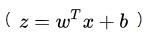 的基础上做分类,比如二分类任务,即
  ,直觉上我们会怎么做?最直观的,可以将线性模型的输出值再套上一个函数
  ,最简单的就是“单位阶跃函数”(unit-step function),如下图中红色线段所示。
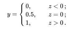
也就是把  看作为一个分割线,大于
 的判定为类别0,小于
的判定为类别1。但是,这样的分段函数数学性质不太好,它既不连续也不可微。我们知道,通常在做优化任务时,目标函数最好是连续可微的。那么如何改进呢?
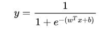
这里就用到了对数几率函数 (形状如图中黑色曲线所示):
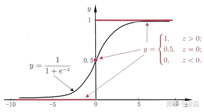
单位阶跃函数与对数几率函数(来源于周志华《机器学习》)
它是一种“Sigmoid”函数,Sigmoid 函数这个名词是表示形式S形的函数,对数几率函数就是其中最重要的代表。这个函数相比前面的分段函数,具有非常好的数学性质,其主要优势如下:
使用该函数做分类问题时,不仅可以预测出类别,还能够得到近似概率预测。这点对很多需要利用概率辅助决策的任务很有用。
对数几率函数是任意阶可导函数,它有着很好的数学性质,很多数值优化算法都可以直接用于求取最优解。
总的来说,模型的完全形式如下:
其实,LR 模型就是在拟合 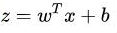 这条直线,使得这条直线尽可能地将原始数据中的两个类别正确的划分开。
1.2 损失函数
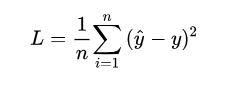
对于任何机器学习问题,都需要先明确损失函数,LR模型也不例外,在遇到回归问题时,通常我们会直接想到如下的损失函数形式 (平均误差平方损失 MSE):
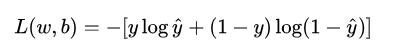
但在 LR 模型要解决的二分类问题中,损失函数式什么样的呢?先给出这个损失函数的形式,可以看一看思考一下,然后再做解释。
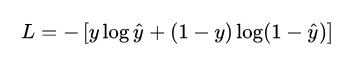
这个损失函数通常称作为 对数损失 (logloss),这里的对数底为自然对数 e ,其中真实值  是有 0/1 两种情况,而推测值
  由于借助对数几率函数,其输出是介于0~1之间连续概率值。仔细查看,不难发现,当真实值
  时,第一项为0,当真实值
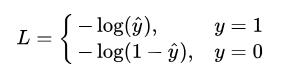
  时,第二项为0,所以,这个损失函数其实在每次计算时永远都只有一项在发挥作用,那这不就可以转换为分段函数了吗,分段的形式如下:
不难发现,当真实值  为1时,输出值
  越接近1,则
  越小,当真实值
  为 0 时,输出值
  越接近于0,则
  越小 (可自己手画一下
  函数的曲线)。该分段函数整合之后就是上面我们所列出的 logloss 损失函数的形式。
1.3 优化求解
现在我们已经确定了模型的损失函数,那么接下来就是根据这个损失函数,不断优化模型参数从而获得拟合数据的最佳模型。
重新看一下损失函数,其本质上是  关于模型中线性方程部分的两个参数
  和
和  的函数:
的函数:
其中, 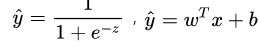
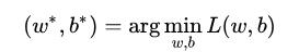
现在的学习任务转化为数学优化的形式即为:
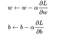
由于损失函数连续可微,我们就可以借助 梯度下降法 进行优化求解,对于连个核心参数的更新方式如下:
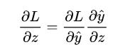
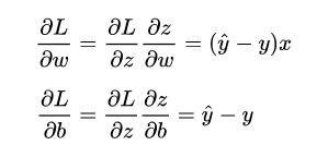
根据求导中的链式法则 :
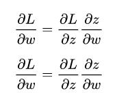
因此,先求解  ,再次使用链式法则:
求得:
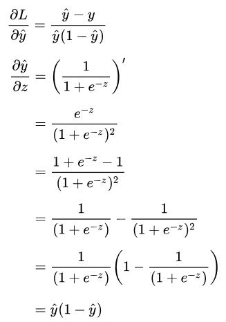
计算到这里,很有意思的事情发生了:
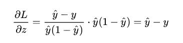
 计算了半天原来变得如此简单,就是推测值
 和真实值
之间的差值,其实这也是得益于对数几率函数本身很好的数学性质。
再接再厉,求得:
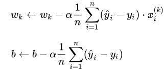
故参数 和
的更新公式如下:
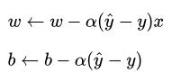
考虑所有样本点  ,计算方法为:
转换为矩阵的计算方式为:
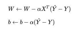
至此,Logistic Regression 模型的优化过程介绍完毕。
2 代码实现
下面我们开始用 python 自己实现一个简单的 LR 模型。
首先,建立 logistic_regression.py 文件,构建 LR 模型的类,内部实现了其核心的优化函数。
# -*- coding: utf-8 -*-

import numpy as np


class LogisticRegression(object):

    def __init__(self, learning_rate=0.1, max_iter=100, seed=None):
        self.seed = seed
        self.lr = learning_rate
        self.max_iter = max_iter

    def fit(self, x, y):
        np.random.seed(self.seed)
        self.w = np.random.normal(loc=0.0, scale=1.0, size=x.shape[1])
        self.b = np.random.normal(loc=0.0, scale=1.0)
        self.x = x
        self.y = y
        for i in range(self.max_iter):
            self._update_step()
            # print('loss: \t{}'.format(self.loss()))
            # print('score: \t{}'.format(self.score()))
            # print('w: \t{}'.format(self.w))
            # print('b: \t{}'.format(self.b))

    def _sigmoid(self, z):
        return 1.0 / (1.0 + np.exp(-z))

    def _f(self, x, w, b):
        z = x.dot(w) + b
        return self._sigmoid(z)

    def predict_proba(self, x=None):
        if x is None:
            x = self.x
        y_pred = self._f(x, self.w, self.b)
        return y_pred

    def predict(self, x=None):
        if x is None:
            x = self.x
        y_pred_proba = self._f(x, self.w, self.b)
        y_pred = np.array([0 if y_pred_proba[i] < 0.5 else 1 for i in range(len(y_pred_proba))])
        return y_pred

    def score(self, y_true=None, y_pred=None):
        if y_true is None or y_pred is None:
            y_true = self.y
            y_pred = self.predict()
        acc = np.mean([1 if y_true[i] == y_pred[i] else 0 for i in range(len(y_true))])
        return acc

    def loss(self, y_true=None, y_pred_proba=None):
        if y_true is None or y_pred_proba is None:
            y_true = self.y
            y_pred_proba = self.predict_proba()
        return np.mean(-1.0 * (y_true * np.log(y_pred_proba) + (1.0 - y_true) * np.log(1.0 - y_pred_proba)))

    def _calc_gradient(self):
        y_pred = self.predict()
        d_w = (y_pred - self.y).dot(self.x) / len(self.y)
        d_b = np.mean(y_pred - self.y)
        return d_w, d_b

    def _update_step(self):
        d_w, d_b = self._calc_gradient()
        self.w = self.w - self.lr * d_w
        self.b = self.b - self.lr * d_b
        return self.w, self.b
然后,这里我们创建了一个 文件,单独用于创建模拟数据,并且内部实现了训练/测试数据的划分功能。
# -*- coding: utf-8 -*-

import numpy as np


def generate_data(seed):
    np.random.seed(seed)
    data_size_1 = 300
    x1_1 = np.random.normal(loc=5.0, scale=1.0, size=data_size_1)
    x2_1 = np.random.normal(loc=4.0, scale=1.0, size=data_size_1)
    y_1 = [0 for _ in range(data_size_1)]
    data_size_2 = 400
    x1_2 = np.random.normal(loc=10.0, scale=2.0, size=data_size_2)
    x2_2 = np.random.normal(loc=8.0, scale=2.0, size=data_size_2)
    y_2 = [1 for _ in range(data_size_2)]
    x1 = np.concatenate((x1_1, x1_2), axis=0)
    x2 = np.concatenate((x2_1, x2_2), axis=0)
    x = np.hstack((x1.reshape(-1,1), x2.reshape(-1,1)))
    y = np.concatenate((y_1, y_2), axis=0)
    data_size_all = data_size_1+data_size_2
    shuffled_index = np.random.permutation(data_size_all)
    x = x[shuffled_index]
    y = y[shuffled_index]
    return x, y

def train_test_split(x, y):
    split_index = int(len(y)*0.7)
    x_train = x[:split_index]
    y_train = y[:split_index]
    x_test = x[split_index:]
    y_test = y[split_index:]
    return x_train, y_train, x_test, y_test
最后,创建 train.py 文件,调用之前自己写的 LR 类模型实现分类任务,查看分类的精度。
# -*- coding: utf-8 -*-

import numpy as np
import matplotlib.pyplot as plt
import data_helper
from logistic_regression import *


# data generation
x, y = data_helper.generate_data(seed=272)
x_train, y_train, x_test, y_test = data_helper.train_test_split(x, y)

# visualize data
# plt.scatter(x_train[:,0], x_train[:,1], c=y_train, marker='.')
# plt.show()
# plt.scatter(x_test[:,0], x_test[:,1], c=y_test, marker='.')
# plt.show()

# data normalization
x_train = (x_train - np.min(x_train, axis=0)) / (np.max(x_train, axis=0) - np.min(x_train, axis=0))
x_test = (x_test - np.min(x_test, axis=0)) / (np.max(x_test, axis=0) - np.min(x_test, axis=0))

# Logistic regression classifier
clf = LogisticRegression(learning_rate=0.1, max_iter=500, seed=272)
clf.fit(x_train, y_train)

# plot the result
split_boundary_func = lambda x: (-clf.b - clf.w[0] * x) / clf.w[1]
xx = np.arange(0.1, 0.6, 0.1)
plt.scatter(x_train[:,0], x_train[:,1], c=y_train, marker='.')
plt.plot(xx, split_boundary_func(xx), c='red')
plt.show()

# loss on test set
y_test_pred = clf.predict(x_test)
y_test_pred_proba = clf.predict_proba(x_test)
print(clf.score(y_test, y_test_pred))
print(clf.loss(y_test, y_test_pred_proba))
# print(y_test_pred_proba)
输出结果图如下:
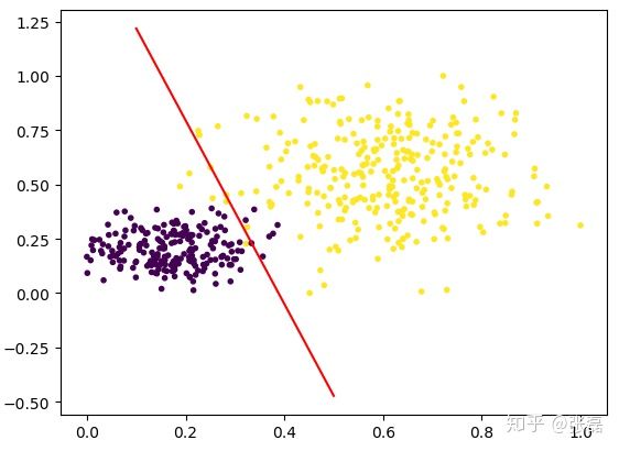
输出的分类结果图
红色直线即为 LR 模型中的线性方程,所以本质上 LR 在做的就是不断拟合这条红色的分割边界使得边界两侧的类别正确率尽可能高。因此,LR 其实是一种线性分类器,对于输入数据的分布为非线性复杂情况时,往往需要我们采用更复杂的模型,或者继续在特征工程上做文章。